How To Install InfluxDB on Windows

How To Install InfluxDB on Windows in 2021 | Installation, Configuration & Running of InfluxDB on Windows

In the present world, technologies are updating day by day with plenty of advanced facilities. Likewise, the installation of InfluxDB on windows tutorials also may differ some time to time. So, here we have come up with a useful and handy tutorial on How To Install InfluxDB on Windows which is good and up-to-date among others.

These types of technologies may change and grow all the time so educational resources should adapt properly. The main objective of offering this tutorial is to have an insightful and up-to-date article on how to install it on Windows.

The tutorial of Install InfluxDB on Windows in 2021 covers the following stuff in a detailed way:

Be ready to follow all the required steps for a clean InfluxDB installation.

How do you install InfluxDB on Windows in 2021?

Check out this video tutorial on how to install InfluxDB on windows and moreover, you can learn the basic commands of influxdb, and integration with Grafana from here:

How to download InfluxDB on Windows?

By following the below two methods, you can easily download the InfluxDB on windows:

a – Downloading the archive

Downloading InfluxDB is very straightforward.

Head over to the InfluxDB downloads page. There, you will see the following four boxes.

a – Downloading the archive

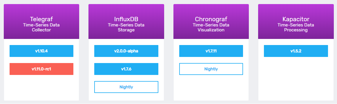
What are those four boxes for?

They are part of the TICK stack. (Telegraf, InfluxDB, Chronograf, and Kapacitor).

Each of these tools has a very specific role: gathering metrics, storing data, visualizing time series or having post-processing defined functions on your data.

In this tutorial, we are going to focus on InfluxDB (the time series database component of TICK)

So should you download the v1.7.6 or v2.0.0 version?

In my previous articles, I answered the main difference between the two versions, but here’s the main difference you need to remember.

features

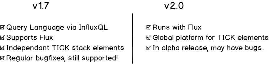
As the 2.0 version is still experimental, we are going to go for the 1.7.6 version.

Click on the v1.7.6 button.

Another window will open with all operating systems. Scroll until you see Windows Binaries (64-bit).

windows-64-bits

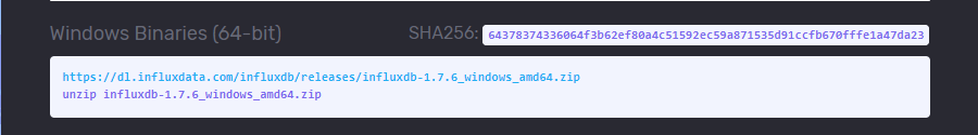
Simply click on the URL in the white box, and the download will automatically start in your browser.

Store it wherever you want, in my case, it will be in the Program Files folder.

Unzip the archive using your favorite archive utility tool (7-Zip in my case) or run the following command in a Powershell command line.

Expand-Archive -Force C:\path\to\archive.zip C:\where\to\extract\to

Great! Let’s take a look at what you have here.

b – Inspecting the archive

Inside your folder, you now have 5 binaries and 1 configuration file:

  • influx.exe: a CLI used to execute IFQL commands and navigate into your databases.
  • influx_inspect.exe: get some information about InfluxDB shards (in a multinode environment)
  • influx_stress.exe: used to stress-test your InfluxDB database
  • influx_tsm.exe: InfluxDB time-structured merge tree utility (not relevant here)
  • influxd.exe: used to launch your InfluxDB server
  • influxdb.conf: used to configure your InfluxDB instance.

Relevant binaries were marked in bold.

Also Check: How To Create a Grafana Dashboard? (UI + API methods)

How to configure InfluxDB Server on your Machine

Before continuing, you have to configure your InfluxDB instance for Windows.

We are essentially interested in four sections in the configuration file.

a – Meta section

This is where your raft database will be stored. It stores metadata about your InfluxDB instance.

Create a meta folder in your InfluxDB directory (remember in my case it was Program Files).

Modify the following section in the configuration file.

[meta]
  # Where the metadata/raft database is stored
  dir = "C:\\Program Files\\InfluxDB\\meta"

b – Data section

InfluxDB stores TSM and WAL files as part of its internal storage. This is where your data is going to be stored on your computer. Create a data and a wal folder in your folder. Again, modify the configuration file accordingly.

[data]
  # The directory where the TSM storage engine stores TSM files.
  dir = "C:\\Program Files\\InfluxDB\\data"

  # The directory where the TSM storage engine stores WAL files.
  wal-dir = "C:\\Program Files\\InfluxDB\\wal

Important: you need to put double quotes in the path!

c – HTTP section

There are many ways to insert data into an InfluxDB database.

You can use client libraries to use in your Python, Java, or Javascript applications. Or you can use the HTTP endpoint directly.

InfluxDB exposes an endpoint that one can use to interact with the database. It is on port 8086. (here’s the full reference of the HTTP API)

Back to your configuration file. Configure the HTTP section as follows:

[http]
  # Determines whether HTTP endpoint is enabled.
  enabled = true

  # The bind address used by the HTTP service.
  bind-address = ":8086"

  # Determines whether HTTP request logging is enabled.
  log-enabled = true

Feel free to change the port as long as it is not interfering with ports already used on your Windows machine or server.

d – Logging section

The logging section is used to determine which levels of the log will be stored for your InfluxDB server. The parameter by default is “info”, but feel free to change it if you want to be notified only for “error” messages for example.

[logging]
  # Determines which log encoder to use for logs. Available options
  # are auto, logfmt, and json. auto will use a more user-friendly
  # output format if the output terminal is a TTY, but the format is not as
  # easily machine-readable. When the output is a non-TTY, auto will use
  # logfmt.
  # format = "auto"

  # Determines which level of logs will be emitted. The available levels
  # are error, warn, info, and debug. Logs that are equal to or above the
  # specified level will be emitted.
  level = "error"

e – Quick test

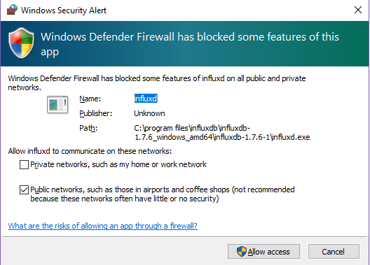
Before configuring InfluxDB as a service, let’s run a quick-dry test to see if everything is okay.

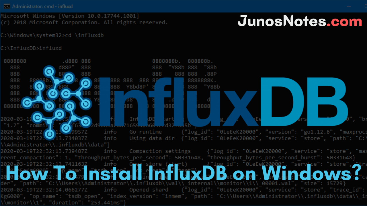
In a command-line, execute the influxd executable. Accept the firewall permission if you are prompted to do it.

firewall

Now that your InfluxDB server has started, start a new command-line utility and run the following command.

C:\Users\Antoine>curl -sl -I http://localhost:8086/ping
HTTP/1.1 204 No Content
Content-Type: application/json
Request-Id: 7dacef6d-8c2f-11e9-8018-d8cb8aa356bb
X-Influxdb-Build: OSS
X-Influxdb-Version: 1.7.6
X-Request-Id: 7dacef6d-8c2f-11e9-8018-d8cb8aa356bb
Date: Tue, 11 Jun 2021 09:58:41 GMT

The /ping endpoint is used to check if your server is running or not.

Are you getting a 204 No Content HTTP response?

Congratulations!

You now simply have to run it as a service, and you will be all done.

How to Run InfluxDB as a Windows service using NSSM Tool?

As you guessed, you are not going to run InfluxDB via the command line every time you want to run it. That’s not very practical.

You are going to run it as a service, using the very popular NSSM tool on Windows.

You could use the SC tool that is natively available on Windows, but I just find it more complicated than NSSM.

To download NSSM, head over to https://nssm.cc/download.

Extract it in the folder that you want, for me, it will be “C:\Program Files\NSSM”.

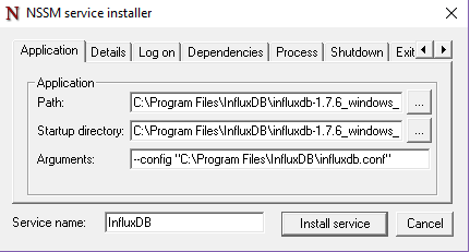
From there, in the current NSSM folder, run the following command (you need administrative rights to do it)

> nssm install

You will be prompted with the NSSM window.

Enter the following details in it (don’t forget the config section, otherwise our previous work is useless)

nssm-config

That’s it!

Now your service is installed.

Head over to the services in Windows 10. Find your service under the name and verify that its status is “Running” (if you specified an automatic startup type in NSSM of course)

Is it running? Let’s verify one more time with curl.

C:\Users\Antoine>curl -sL -I http://localhost:8086/ping
HTTP/1.1 204 No Content
Content-Type: application/json
Request-Id: ef473e13-8c38-11e9-8005-d8cb8aa356bb
X-Influxdb-Build: OSS
X-Influxdb-Version: 1.7.6
X-Request-Id: ef473e13-8c38-11e9-8005-d8cb8aa356bb
Date: Tue, 11 Jun 2021 11:06:17 GMT

Congratulations! You did it!

You installed InfluxDB on Windows as a service, and it is running on port 8086.

Most Common Mistakes In The Process

The service did not respond in a timely fashion.

I encountered this error when I tried to set up InfluxDB as a service using SC. As many solutions exist on Google and on Youtube, I solved it by using NSSM.

Tried tweaking the Windows registry but it wasn’t very useful at all.

Only one usage of each socket address (protocol/network address/port) is normally permitted.

Simple, there is already a program or service listening on 8086. You should modify the default port in the configuration file and take one that is permitted and not used.

I don’t have the same curl response

A 204 response to the curl command is the only sign that your InfluxDB is running correctly. If you don’t get the same output, you should go back and double-check the steps before.

I have a parsing error in my configuration file!

Remember that in Windows systems backslashs have to be escaped. It’s double backslashs in the paths of your InfluxDB configuration file.

If your path contains some spaces, like “Program Files”, make sure to put your path into quotes.

The Definitive Guide to Centralized Logging with Syslog on Linux

The Definitive Guide to Centralized Logging with Syslog on Linux

One of the important components of any software or Operating system is Logs. In case, you deal mostly with a Linux system administration, then apparently you spend a lot of time browsing your log files to obtain appropriate data regarding prior events. Generally, it records users’ actions, network activity, system events, and many more based on what they are intended for.

Rsyslog is one of the most extensively used logging systems on Linux OS. It is a very powerful, secure, and high-performance log processing system that accepts information from various types of sources and outputs it into different formats.

In this definitive guide, we are going to explain all How to Centralized Logging with Syslog on Linux Systems. Not just in a brief way, we will be discussing it even more broadly with every single step that you need to put in place to build a reliable, secure, and functional centralized logging system.

Are you ready to experience it practically by referring to this useful tutorial? Go for it:

What is Centralized Logging?

Centralized logging lets you store your Linux, UNIX, and Windows logs in a centralized repository. It also provides several advantages such as:

  • Single location to check for system errors (ever had a disk die that disrupted local logging?)
  • Security, especially when you need to put together timelines after a system compromise
  • Often required for security compliance

What is Syslog‐ng?

Syslog‐ng is a flexible and robust open-source syslog implementation. Syslog-ng offers various advantages for users like as mentioned below:

  • Logging via UDP or TCP
  • Mutual authentication through digital certificates
  • Messages can be parsed and rewritten ( this is especially useful for removing sensitive data from log messages)
  • Encryption of log traffic via TLS
  • Logs can be sent to a SQL database
  • Filters can be used to sort traffic based on host, facility, log level, message contents, etc.

Do Check: Syslog: The Complete System Administrator Guide

What You Will Learn?

As always, let’s start by having a look at everything that you are going to learn if you follow the tutorial until the end.

With this tutorial, you are going to learn:

  • How Linux logging works on a single instance, where to look after logs;
  • What a centralized logging architecture looks like advantages and drawbacks of using it;
  • How to setup rsyslog forwarding from a client to a centralized server;
  • How to secure log forwarding using the TLS protocol;
  • How to send logs using reliable mechanisms such as action queues.

That’s a long program, but feel free to skip some sections if you are already comfortable with some of the concepts explained in this article.

How does Linux logging works on a single instance?

Let’s start with a bit of history about Linux logging.

a – General concepts of Linux logging

Before jumping into building our centralized logging architecture, there are some concepts about logging on a single instance that are mandatory to understand more complex concepts.

By default, your Linux operating system records logs about many events that are happening on your machine.

Linux uses the syslog protocol which defines a standard for every aspect of logging on an operating system (not only Linux but also Windows): defining what a message looks like, describing severity levels on messages, as well as listing the ports that syslog will be using.

Syslog can be used as a server (hosting the logs) or as a client (forwarding the logs to a remote server).

As a consequence, the syslog protocol also defines how to log transmission should be done, both in a reliable and secure way.

If you are using a modern Linux distribution (like a Ubuntu machine, a CentOS, or an RHEL one), the default syslog server used is rsyslog.

rsyslog-card

Rsyslog comes as an evolution of syslog, providing capabilities such as configurable modules that can be bound to a wide variety of targets (forwarding Apache logs to a remote server for example).

Rsyslog also provides native filtering as well as templates to format data to a custom format.

b – Where are logs stored on a Linux filesystem?

Long story short, logs are stored at /var/log/ on your filesystem.

At this location, you should see multiple log files, each one having a name describing what they actually store.

For a quick overview, you can execute the following command:

$ ls -l /var/log
-rw-r-----  1 syslog        adm               120999 Jul 24 18:04 auth.log
-rw-r--r--  1 root          root              127503 Jul 20 06:35 dpkg.log
-rw-r-----  1 syslog        adm                    0 Jul 15 06:25 kern.log
drwxrwxr-x  2 logstash      root                4096 Jul  8 18:33 logstash
drwxr-xr-x  2 root          root                4096 Sep 10  2018 lxd
drwxr-xr-x  2 mongodb       mongodb             4096 Jul  8 06:25 mongodb

As you can see, you have dedicated log files for authentication purposes or for kernel related logs.

/var/log does not contain only files, but it also contain dedicated folders that vendors create when the application is installed.

As you can see, I am running a MongoDB database on my instance.

As a consequence, I have a MongoDB folder in my log folder.

But why am I telling you all of this?

Because using this knowledge, we are going to lay the first brick of your centralized logging architecture.

Suppose that three machines are sending logs to my server, each machine is going to have its own own auth.log, kern.log or dpkg.log files.

As a consequence, you want logs to be stored in dedicated folders, one for each instance.

Here’s the folder architecture on the server side.

centralized-folder-architecture

Designing a centralized logging architecture on Linux

Now that we have the basics of Linux logging, we are ready to design a centralized logging architecture.

As described in the first section, every machine in our pool is already writing logs via rsyslog.

However, natively, our machines are configured as client-server syslog instances.

They create logs, but they store them locally in the file system.

On our centralized logging architecture, client machines will be configured to use rsyslog as a client, and they will forward every single log to a remote rsyslog server, which is the central server.

logging-architecture-1

To be complete, our architecture has to:

  • Be secure : that’s why we are going to implement TLS in the fifth section;
  • Be reliable : if the entire network goes down for a minute, are all logs for this period lost forever? Not with action queues.

What are the advantages of such an architecture?

  • You can inspect all your logs from a single place : you don’t rely on connecting individually to every machine on your pool, you can directly see the logs from the same filesystem.
  • You have access to logs, even if the host is not accessible : if one of the machines is having issues and it cannot be reached, you would not be able to go through the filesystem to look after logs. With a centralized logging server, you have the opportunity to look at logs, without any physical access to the client machine.
  • You can set up a complete log monitoring infrastructure : if you are interested in visualizing your logs with tools such as Kibana, I wrote a complete guide about it.

On the other hand, what would be for us the drawbacks of such an architecture?

  • You risk overloading your syslog server : with this architecture, you are pushing logs to a remote server. As a consequence, if one machine goes crazy and starts sending thousands of logs, you risk overloading the log server. (if you want a reliable back-pressure control, you can check Filebeat by Elastic)
  • If your log server goes down, you lose the ability to look at all the logs sent by the clients. Moreover, if the server goes down, clients will start storing messages locally until the server is available again, thus filling up disk space on the client side.

Configure rsyslog to forward logs to a centralized server

Prerequisites

First, make sure that you have rsyslog on your instance.

$ sudo systemctl status rsyslog

rsyslog-service

If the service is unknown on your computer, you can install it by running:

$ sudo apt-get update && apt-get install rsyslog
$ sudo systemctl enable rsyslog
$ sudo systemctl start rsyslog

a – Configure your rsyslog server

First of all, you have to configure your rsyslog server for it to accept incoming logs on port 514.

We are going to use TCP for log transmission, but you can use UDP if you don’t care that much about reliability.

On the server, head to /etc/rsyslog.d folder.

This is the directory that stores templates as well as files that contain the rsyslog rules.

In this directory, there should be a 50-default.conf file.

We are going to create our own configuration file, prefixing it with a number lower than the configuration file one.

This way, our configuration file takes priority over the default one.

$ sudo touch 01-server.conf

# Listen for TCP
$ModLoad imtcp
# Listen on port 514
$InputTCPServerRun 514

$template RemoteServer, "/var/log/%HOSTNAME%/%SYSLOGFACILITY-TEXT%.log"
*.* ?RemoteServer
Our first rule!

rsyslog-syntax

With this syntax, our log files will be grouped by hostname (aka the computer name sending the log) and then by syslog facility (kern, user, auth, etc..)

Restart your rsyslog server, and make sure that it is now listening on port 514 for TCP

$ sudo systemctl restart rsyslog
$ netstat -tna | grep :514
tcp        0      0 0.0.0.0:514             0.0.0.0:*               LISTEN
tcp6       0      0 :::514                  :::*                    LISTEN<

Note:  With this configuration file, your server logs are now no longer directly stored in /var/log, but in /var/log/hostname, hostname is the current name of your host (in my case /var/log/schkn-ubuntu)

$ uname -a
Linux schkn-ubuntu 4.15.0-42-generic #45-Ubuntu SMP Thu Nov 15 19:32:57 UTC 2018 x86_64 x86_64 x86_64 GNU/Linux

b – Configure your rsyslog client

It is time to configure rsyslog as a client on our instance.

Now that we have rsyslog, head over to /etc/rsyslog.d.

Similar to the procedure done on the server-side create a 01-client.conf file.

$ sudo vi 01-client.conf

*.*                         @@distant-server-ip:514

The configuration on the client-side is pretty simple, plain simple forwarding.

Restart your rsyslog server, and make sure that:

  • You have no errors on the client-side
$ sudo systemctl restart rsyslog
$ journalctl -f -u rsyslog
  • Your server now has the logs from the client

My client machine is named “antoine-Virtualbox” in my current setup, so I am looking for /var/log/antoine-Virtualbox.

b – Configure your rsyslog client

Awesome! Distant logs are now correctly stored on our server.

However, I have some bad news for you.

As we are using TCP for log transmission, it means that messages are not encrypted between the client and the server.

As a consequence, any hacker that sniffs the packets on your network will be able to see your logs, spy on their content, and perform attacks on your host machines.

This is what we call a man-in-the-middle attack.

As proof, here’s a Wireshark instance sniffing my network and listening for a very specific IP.

clear-message-2

As you can see, the message is clearly visible and states: “Hi, this is a test message”.

Now imagine if the log message contained sensitive information about your host, that could be a complete security disaster.

This is why we are going to setup TLS, allowing us to encrypt the traffic between the client and the server.

At the end of the next chapter, I will provide you with a Wireshark screenshot, proving that the traffic is now encrypted.

Ready?

Encrypting rsyslog messages with TLS

In order for us to encrypt messages between the server and the client, we are going to use TLS and more precisely trusted certificates.

Without going into too many details, those trusted certificates will ensure that both client and server identities are verified.

With this protocol, the client and the server will first ensure that they are correctly talking to each other (as there is no one along the way with a fake identity), and then they will proceed to encrypt their messages.

As the client and the server exchanged their keys, they are able to decrypt messages on the fly.

In our setup, we will have a certificate authority signing the keys.

Communication between the hosts and the certificate authority is obviously encrypted too, so we need first to create a key pair for the certificate authority.

V – Encrypting rsyslog messages with TLS tls-schema

If you are just testing out, you can use your rsyslog server as a certificate authority.

a – Configuring your certificate authority

On the server, head over to /etc/ssl, and create a rsyslog directory.

$ sudo mkdir /etc/ssl/rsyslog
$ cd /etc/ssl/rsyslog

Install the gnutls-utils package (that might come as the gnutls-bin for some distributions) that enables SSL API on your server.

$ sudo apt-get install gnutls-utils
(or)
$ sudo apt-get install gnutls-bin

Generate a private key for the certificate authority:

$ sudo certtool --generate-privkey --outfile CA-key.pem
$ sudo chmod 400 CA-key.pem

Generate a public key on the certificate authority:

$ sudo certtool --generate-self-signed --load-privkey CA-key.pem --outfile CA.pem
# Common name: authority.devconnected.com
  # The certificate will expire in (days): 3650
  # Does the certificate belong to an authority? (Y/N): y
  # Will the certificate be used to sign other certificates? (Y/N): y
  # Will the certificate be used to sign CRLs? (y/N): y

You can leave the other questions blank as they will have no impact on the final result.

b – Generating private/public keys for the server

Now that our certificate authority has keys to sign other keys, let’s create one for the rsyslog server.

First, create a private key for your server.

$ sudo certtool --generate-privkey --outfile server-key.pem --bits 2048

Generate a certificate request for your server.

$ sudo certtool --generate-request --load-privkey server-key.pem --outfile server-request.pem

Generate the certificate for your rsyslog server and import trusted certificate authority keys into it.

$ sudo certtool --generate-certificate --load-request server-request.pem --outfile server-cert.pem --load-ca-certificate CA.pem --load-ca-privkey CA-key.pem

  # The certificate will expire in (days): 3650
  # Is this a TLS web client certificate? (Y/N): y
  # Is this also a TLS web server certificate? (y/N): y
  # Enter a dnsName of the subject of the certificate: server.devconnected.com

c – Generate private/public keys for the client

Similar to what we have done before, let’s build our key pair for the client.

Create a private key for the client.

$ sudo certtool --generate-privkey --outfile client-key.pem --bits 2048

Generate a certificate request for the client.

$ sudo certtool --generate-request --load-privkey client-key.pem --outfile client-request.pem

Create a certificate (a public key) for your client and import the certificate authority certificates inside.

$ sudo certtool --generate-certificate --load-request client-request.pem --outfile client-cert.pem --load-ca-certificate CA.pem --load-ca-privkey CA-key.pem

# The certificate will expire in (days): 3650
  # Is this a TLS web client certificate? (Y/N): y
  # Is this also a TLS web server certificate? (y/N): y
  # Enter a dnsName of the subject of the certificate: client.devconnected.com

Awesome! We now have key pairs for both our client and server.

d – Send generated keys to your hosts

Now that your keys are generated on the certificate authority, send your keys securely to the destination hosts.

For this, you can use scp.

For the server (simply switch to ‘client’ when you want to send keys to the client)

$ sudo -u root scp -i ~/.ssh/id_rsa CA.pem server-* root@server_ip_here:/etc/ssl/rsyslog/

e – Configure your rsyslog server

Now that both servers and clients contain keys for encryption, let’s configure hosts to conclude this chapter.

First, install the gtls driver on your server.

$ sudo apt-get install rsyslog-gnutls

As a reminder, we create a 01-server.conf file in the previous chapter.

Replace the content with the following configuration.

# Listen for TCP
$ModLoad imtcp
# GTLS driver
$DefaultNetstreamDriver gtls
# Certificates
$DefaultNetstreamDriverCAFile /etc/ssl/rsyslog/CA.pem
$DefaultNetstreamDriverCertFile /etc/ssl/rsyslog/server-cert.pem
$DefaultNetstreamDriverKeyFile /etc/ssl/rsyslog/server-key.pem
# Authentication mode
$InputTCPServerStreamDriverAuthMode x509/name
$InputTCPServerStreamDriverPermittedPeer *.devconnected.com
# Only use TLS
$InputTCPServerStreamDriverMode 1
# Listen on port 514
$InputTCPServerRun 514

$template RemoteServer, "/var/log/%HOSTNAME%/%SYSLOGFACILITY-TEXT%.log"
*.* ?RemoteServer

As you can see, we are adding an AuthMode, which is x509/name in this case.

This means that we are going to use a certificate that contains a “name” inside it.

Remember when we declare that we were “client.devconnected.com” or “server.devconnected.com” when we created the certificates?

This is exactly the information that the authentication is going to use, and you will get an error if the name does not match.

Don’t forget to restart rsyslog for the changes to be saved.

$ sudo systemctl restart rsyslog

f – Configure your rsyslog client

On the client, we had a simple forwarding rule in a 01-client.conf file.

Again, install the gtls driver on your client.

$ sudo apt-get install rsyslog-gnutls

Replace the content with the following configuration.

# GTLS driver
$DefaultNetstreamDriver gtls
# Certificates
$DefaultNetstreamDriverCAFile /etc/ssl/rsyslog/CA.pem
$DefaultNetstreamDriverCertFile /etc/ssl/rsyslog/client-cert.pem
$DefaultNetstreamDriverKeyFile /etc/ssl/rsyslog/client-key.pem
# Auth mode
$ActionSendStreamDriverAuthMode x509/name
$ActionSendStreamDriverPermittedPeer server.devconnected.com
# Only use TLS
$ActionSendStreamDriverMode 1
# Forward everything to server.devconnected.com
*.* @@distant-server-ip:514

Restart your rsyslog client.

$ sudo systemctl restart rsyslog

Awesome! Your logs should now be sent to your remote server. Run this command and make sure that you have no errors (if you do, I have a section for it at the end)

$ $ journalctl -u -n 100 rsyslog

A promise is a promise, here’s my Wireshark between my server and my client, with a TLS encryption between them.

encrypted-2

No way for you to decrypt the message.

Plot twist : I sent “Hi, this is a test message” again.

Sending log messages reliably with action queues

In the architecture that we designed before, there is one major issue that was not addressed before: reliability.

In our architecture, the client and the server are very tightly coupled.

What does it mean?

If the server goes down, your client will obviously not be able to send log messages, but they might also risk losing the logs messages forever.

error-losing-server-1

Luckily for us, rsyslog has a contingency plan when it comes to bad forwarding: plain and simple disabling the faulty module.

module-disabled-1

This means that you won’t lose your messages (they still be stored locally), but you are losing your log forwarding altogether.

Would you go back to your host to re-enable your forwarding module every time the network goes down? I wouldn’t.

To solve this, we need to bring decoupling to this architecture.

If you read the Entreprise Integration Patterns book by Gregor Hohpe, reliability means queues.

decoupled-arch-2

a – Designing message reliability

First, let’s understand a couple of concepts related to rsyslog message queues.

rsyslog-queues

In rsyslog, there are multiple ways for you to design queues, but eventually, it comes up the three main categories:

  • Direct: this is kind of a “no queue” mode where messages are directly passed from the producer to the consumer. Definitely not a mode we want to be implemented in our case;
  • Disk queues: in this case, as messages are passed to the queue, they are reliably written to the disk. In this case, you are safer when it comes to machine complete accidental shutdown, but the process is longer than memory queues. Writing to disk is more expensive than writing in the RAM;
  • Memory queues: those queues will hold messages in memory for a given time and for a given amount of restricted space. After a while, they will be written to disk. This alternative is faster than disk queues.

For our architecture, we are going to use memory queues with a bunch of different options (all options are available here)

In your 01-client.conf file, append the following lines to your configuration file.

$ActionQueueType LinkedList
$ActionQueueFileName rsyslog_backup
$ActionQueueSaveOnShutdown on
$ActionResumeRetryCount -1
...
# Parameters from the TLS section
$ActionSendStreamDriverAuthMode x509/name
  • LinkedList: we want memory allocation to be done on the fly, and not via a fixed array. This will create more overhead computation but you will benefit from it by gaining more space;
  • Queue file name: this is the file where data is going to be written if data is eventually stored to disk. The path to it is $WorkDirectory/rsyslog_backup where WorkDirectory is the variable defined in your rsyslog.conf file;
  • Save on shutdown: if the machine was to shut down, the memory logs would be written to disk first;
  • Resume retry count: when losing the forwarding module, rsyslog will try to reconnect to it indefinitely.

You can tweak it more given the specifications you are working with, but I will go with that for this tutorial.

Restart rsyslog, and make sure that you are not having any errors.

$ sudo systemctl restart rsyslog
$ sudo journalctl -f -u rsyslog.service

b – Demonstrating message reliability

Okay, now that we have message reliability put in place, let’s test it out.

On the server-side, comment all the lines in your 01-server.conf file and restart rsyslog. From this point, your client should lose its connection to the server.

On the client:

$ sudo journalctl -f -u rsyslog.service

client-losing-connection

On the client, manually fire a log event.

$ logger -p 'auth.crit' 'Critial auth message, lost?'

Verify that you are not receiving anything at all on the server and that the client does not fire any preemptive message.

From there, your message is stored in memory, patiently waiting for the module to be back up.

Go to the server-side, remove comments for all the lines, and restart your rsyslog server.

From there, your client will automatically re-enable the forwarding module.

client-module-back-up

But, did our server receive the message that was stored in the client’s memory? It did!

server-received-message

Congratulations, you designed (secure!) message reliability between rsyslog clients and a rsyslog server.

Common Errors

Here is a list of the different errors that you may encounter during the process:

  • omfwd: TCPSendBuf error -2027, destruct TCP connection the x.x.x.x

error-1-ssl-1

Solution: if you are having this error in the TLS section, your TLS configuration is probably wrong. Either you have badly configured the certificates, or you have the wrong server configuration.

  • Cannot connect to x.x.x.x : network is unreachable.

error-2-network-unreachable

Solution: make sure that the IP address can be accessed from the client host. You can ping it by example.

$ ping 142.93.103.142
PING 142.93.103.142 (142.93.103.142) 56(84) bytes of data.
64 bytes from 142.93.103.142: icmp_seq=1 ttl=64 time=0.023 ms
64 bytes from 142.93.103.142: icmp_seq=2 ttl=64 time=0.056 ms
64 bytes from 142.93.103.142: icmp_seq=3 ttl=64 time=0.033 ms
--- 142.93.103.142 ping statistics ---
3 packets transmitted, 3 received, 0% packet loss, time 2047ms
  • Peer name not authorized: not permitted to talk to it. Names CN: name.domain.com

error-3-not-correct-host

In the rsyslog configuration file, make sure that you have the $ActionSendStreamDriverPermittedPeers correctly set.

Bonus: A word on back-pressure protocols

Before ending this guide, there is one point that I want to address, as I think that it might be something that could be improved in this architecture.

a – Architectural improvements

The architecture that we designed together can be seen as a “push” architecture. We essentially push logs from the client to the servers.

And that’s risky.

Why?

Because if the clients begin to send too many logs files to your server, you have the risks of overloading your entire system, preventing other clients to send data. From there, it is only a matter of time until your server goes down, or until you start losing logs files completely.

Here are some thoughts about how to handle this:

  • Use the dequeueSlowDown rsyslog parameter to delay message execution, essentially putting a tempo on all the messages being sent. Here is a link to it.
  • Use a back-pressure third-party product like Filebeat. Filebeat can be interesting if you are already working with the ELK stack all together. It implements a native back-pressure protocol for you to set a rate on when the logs are being sent.

b – Push vs Pull logging systems

We have already tackled the difference between push and pull systems at least when it comes to open source monitoring solutions.

We have seen the advantage of building an active monitoring solution, but couldn’t we apply the same principles when it comes to centralized logging systems?

As our log files are stored in disks, there is definitely a way for us to parse those files regularly and extract logs, at a rate that we decide on the server-side. This point removes the danger of having a client overloading our servers.

push-vs-pull

Are you aware of a system that is designed this way?

Conclusion

This last point ends this definitive guide about centralized logging for Linux systems.

In this guide, we went through pretty much all the aspects of centralized logging: from one single instance, to log forwarding to a central server in a secure and reliable way.

If you really want to go further on the subject, here are some videos that are related to the subjects, and that I found interesting.

Monitoring Linux Logs with Kibana and Rsyslog

Monitoring Linux Logs with Kibana and Rsyslog | Using Kibana and Rsyslog to monitor Linux logs

A system administrator and enthusiastic application developers can grab this best opportunity of digging deep into this tutorial and acquire the complete details about Monitoring Linux Logs with Kibana and Rsyslog along with how to build a monitoring pipeline to analyze Linux logs with ELK 7.2 and Rsyslog.

If you are curious to learn solutions for such queries as monitoring SSH intrusions on VMs, observing what errors were raised by your application server on a special day, on a very special hour, or else you need to check a few insights regarding who stopped your systemd service on one of your VMs.

In case, you have raised even one of these questions in your mind while working on Linux logs then you are on the right site.

So, concentrate on this entire tutorial where you will get to know how to build a complete log monitoring pipeline using the ELK stack (ElasticSearch, Logstash, and Kibana) and Rsyslog as a powerful Syslog server.

As you know that you are on the right page, but before going to learn the main concepts or directly go through the technical considerations right away, let’s have a talk about why do we want to monitor Linux logs with Kibana.

Why should you monitor Linux logs?

Monitoring Linux logs is crucial and every DevOps engineer should know how to do it. Here’s why :

  • You have real-time visual feedback about your logs: probably one of the key aspects of log monitoring, you can build meaningful visualizations (such as data tables, pies, graphs, or aggregated bar charts) to give some meaning to your logs.
  • You are able to aggregate information to build advanced and more complex dashboards: sometimes raw information is not enough, you may want to join it with other logs or to compare it with other logs to identify a trend. A visualization platform with expression handling lets you perform that.
  • You can quickly filter for a certain term, or given a certain time period: if you are only interested in SSH logs, you can build a targeted dashboard for it.
  • Logs are navigable in a quick and elegant way: I know the pain of tailing and grepping your logs files endlessly. I’d rather have a platform for it.

why-log-monitoring

What You Will Learn?

There are many things that you are going to learn if you follow this tutorial:

  • How logs are handled on a Linux system (Ubuntu or Debian) and what rsyslog is.
  • How to install the ELK stack (ElasticSearch 7.2, Logstash, and Kibana) and what those tools will be used for.
  • How to configure rsyslog to forward logs to Logstash
  • How to configure Logstash for log ingestion and ElasticSearch storage.
  • How to play with Kibana to build our final visualization dashboard.

tools-for-log-monitoring

The prerequisites for this tutorial are as follows :

  • You have a Linux system with rsyslog installed. You either have a standalone machine with rsyslog, or a centralized logging system.
  • You have administrator rights or you have enough rights to install new packages on your Linux system.

Without further due, let’s jump into it!

What does a log monitoring architecture look like?

a – Key concepts of Linux logging

Before detailing how our log monitoring architecture looks like, let’s go back in time for a second.

Historically, Linux logging starts with syslog.

Syslog is a protocol developed in 1980 which aims at standardizing the way logs are formatted, not only for Linux but for any system exchanging logs.

From there, syslog servers were developed and were embedded with the capability of handling syslog messages.

Do Check: Syslog: The Complete System Administrator Guide

They rapidly evolved to functionalities such as filtering, having content routing abilities, or probably one of the key features of such servers: storing logs and rotating them.

Rsyslog was developed keeping this key functionality in mind: having a modular and customizable way to handle logs.

The modularity would be handled with modules and the customization with log templates.

In a way, rsyslog can ingest logs from many different sources and it can forward them to an even wider set of destinations. This is what we are going to use in our tutorial.

b – Building a log monitoring architecture

Here’s the final architecture that we are going to use for this tutorial.

  • rsyslog: used as an advancement Syslog server, rsyslog will forward logs to Logstash in the RFC 5424 format we described before.
  • Logstash: part of the ELK stack, Logstash will transform logs from the syslog format to JSON. As a reminder, ElasticSearch takes JSON as an input.
  • ElasticSearch: the famous search engine will store logs in a dedicated log index (logstash-*). ElasticSearch will naturally index the logs and make them available for analysis.
  • Kibana: used as an exploration and visualization platform, Kibana will host our final dashboard.

log-monitoring-architecture

Now that we know in which direction we are heading, let’s install the different tools needed.

Installing The Different Tools

tools-used

a – Installing Java on Ubuntu

Before installing the ELK stack, you need to install Java on your computer.

To do so, run the following command:

$ sudo apt-get install default-jre

At the time of this tutorial, this instance runs the OpenJDK version 11.

ubuntu:~$ java -version
openjdk version "11.0.3" 2019-04-16
OpenJDK Runtime Environment (build 11.0.3+7-Ubuntu-1ubuntu218.04.1)
OpenJDK 64-Bit Server VM (build 11.0.3+7-Ubuntu-1ubuntu218.04.1, mixed mode, sharing)

b – Adding Elastic packages to your instance

For this tutorial, I am going to use a Ubuntu machine but details will be given for Debian ones.

First, add the GPG key to your APT repository.

$ wget -qO - https://artifacts.elastic.co/GPG-KEY-elasticsearch | sudo apt-key add -

Then, you can add Elastic source to your APT source list file.

$ echo "deb https://artifacts.elastic.co/packages/7.x/apt stable main" | sudo tee -a /etc/apt/sources.list.d/elastic-7.x.list

$ cat /etc/apt/sources.list.d/elastic-7.x.list
deb https://artifacts.elastic.co/packages/7.x/apt stable main

$ sudo apt-get update

From there, you should be ready to install every tool in the ELK stack.

Let’s start with ElasticSearch.

c – Installing ElasticSearch

ElasticSearch is a search engine built by Elastic that stores data in indexes for very fast retrieval.

To install it, run the following command:

$ sudo apt-get install elasticsearch

The following command will automatically :

  • Download the deb package for ElasticSearch;
  • Create an elasticsearch user;
  • Create an elasticsearch group;
  • Automatically create a systemd service fully configured (inactive by default)

elastic-service

At the first start, the service is inactive, start it and make sure that everything is running smoothly.

$ sudo systemctl start elasticsearch
● elasticsearch.service - Elasticsearch
   Loaded: loaded (/usr/lib/systemd/system/elasticsearch.service; disabled; vendor preset: enabled)
   Active: active (running) since Mon 2019-07-08 18:19:45 UTC; 2 days ago
     Docs: http://www.elastic.co

In order to make sure that ElasticSearch is actually running, you can execute one of those two commands:

  • Watching which applications listen on a targeted port
$ sudo lsof -i -P -n | grep LISTEN | grep 9200
java      10667   elasticsearch  212u  IPv6 1159208890      0t0  TCP [::1]:9200 (LISTEN)
java      10667   elasticsearch  213u  IPv6 1159208891      0t0  TCP 127.0.0.1:9200 (LISTEN)
  • Executing a simple ElasticSearch query
$ curl -XGET 'http://localhost:9200/_all/_search?q=*&pretty'

Your ElasticSearch instance is all set!

Now, let’s install Logstash as our log collection and filtering tool.

Let’s gain some more knowledge on Elasticsearch by clicking here: How To Install an Elasticsearch Cluster on Ubuntu 18.04

d – Installing Logstash

If you added Elastic packages previously, installing Logstash is as simple as executing:

$ sudo apt-get install logstash

Again, a Logstash service will be created, and you need to activate it.

$ sudo systemctl status logstash
$ sudo systemctl start logstash

By default, Logstash listens for metrics on port 9600. As we did before, list the open ports on your computer looking for that specific port.

$ sudo lsof -i -P -n | grep LISTEN | grep 9600
java      28872        logstash   79u  IPv6 1160098941      0t0  TCP 127.0.0.1:9600 (LISTEN)

Great!

We only need to install Kibana for our entire setup to be complete.

e – Installing Kibana

As a reminder, Kibana is the visualization tool tailored for ElasticSearch and used to monitor our final logs.

Not very surprising, but here’s the command to install Kibana:

$ sudo apt-get install kibana

As usual, start the service and verify that it is working properly.

$ sudo systemctl start kibana
$ sudo lsof -i -P -n | grep LISTEN | grep 5601
node       7253          kibana   18u  IPv4 1159451844      0t0  TCP *:5601 (LISTEN)

Kibana Web UI is available on port 5601.

Head over to http://localhost:5601 with your browser and you should see the following screen.

kibana-welcome-page

Nice!

We are now very ready to ingest logs from rsyslog and to start visualizing them in Kibana.

Routing Linux Logs to ElasticSearch

As a reminder, we are routing logs from rsyslog to Logstash and those logs will be transferred to ElasticSearch pretty much automatically.

a – Routing from Logstash to ElasticSearch

how-does-logstash-work

Before routing logs from rsyslog to Logstash, it is very important that we setup log forwarding between Logstash and ElasticSearch.

To do so, we are going to create a configuration file for Logstash and tell it exactly what to do.

To create Logstash configuration files, head over to /etc/logstash/conf.d and create a logstash.conf file.

Inside, append the following content:

input {                                                                                      
  udp {                                                                                      
    host => "127.0.0.1"                                                                      
    port => 10514                                                                            
    codec => "json"                                                                          
    type => "rsyslog"                                                                        
  }                                                                                          
}                                                                                            
                                                                                             
                                                                            
# The Filter pipeline stays empty here, no formatting is done.                                                                                           filter { }                                                                                   
                                                                                             
                   
# Every single log will be forwarded to ElasticSearch. If you are using another port, you should specify it here.                                                                                             
output {                                                                                     
  if [type] == "rsyslog" {                                                                   
    elasticsearch {                                                                          
      hosts => [ "127.0.0.1:9200" ]                                                          
    }                                                                                        
  }                                                                                          
}

Note: For this tutorial, we are using the UDP input for Logstash, but if you are looking for a more reliable way to transfer your logs, you should probably use the TCP input. The format is pretty much the same, just change the UDP line to TCP.

Restart your Logstash service.

$ sudo systemctl restart logstash

To verify that everything is running correctly, issue the following command:

$ netstat -na | grep 10514
udp        0      0 127.0.0.1:10514         0.0.0.0:*
Great!

Logstash is now listening on port 10514.

b – Routing from rsyslog to Logstash

how-rsyslog-work

As described before, rsyslog has a set of different modules that allow it to transfer incoming logs to a wide set of destinations.

Rsyslog has the capacity to transform logs using templates. This is exactly what we are looking for as ElasticSearch expects JSON as an input, and not syslog RFC 5424 strings.

In order to forward logs in rsyslog, head over to /etc/rsyslog.d and create a new file named 70-output.conf

Inside your file, write the following content:

# This line sends all lines to defined IP address at port 10514
# using the json-template format.

*.*                         @127.0.0.1:10514;json-template

Now that you have log forwarding, create a 01-json-template.conf file in the same folder, and paste the following content:

template(name="json-template"
  type="list") {
    constant(value="{")
      constant(value="\"@timestamp\":\"")     property(name="timereported" dateFormat="rfc3339")
      constant(value="\",\"@version\":\"1")
      constant(value="\",\"message\":\"")     property(name="msg" format="json")
      constant(value="\",\"sysloghost\":\"")  property(name="hostname")
      constant(value="\",\"severity\":\"")    property(name="syslogseverity-text")
      constant(value="\",\"facility\":\"")    property(name="syslogfacility-text")
      constant(value="\",\"programname\":\"") property(name="programname")
      constant(value="\",\"procid\":\"")      property(name="procid")
    constant(value="\"}\n")
}

As you probably guessed, for every incoming message, rsyslog will interpolate log properties into a JSON formatted message, and forward it to Logstash, listening on port 10514.

Restart your rsyslog service, and verify that logs are correctly forwarded to ElasticSearch.

Note: logs will be forwarded in an index called logstash-*.

$ sudo systemctl restart rsyslog
$ curl -XGET 'http://localhost:9200/logstash-*/_search?q=*&pretty'
{
  "took": 2,
  "timed_out": false,
  "_shards": {
    "total": 1,
    "successful": 1,
    "skipped": 0,
    "failed": 0
  },
  "hits": {
    "total": {
      "value": 10000,
      "relation": "gte"
    },
    "max_score": 1,
    "hits": [
      {
        "_index": "logstash-2019.07.08-000001",
        "_type": "_doc",
        "_id": "GEBK1WsBQwXNQFYwP8D_",
        "_score": 1,
        "_source": {
          "host": "127.0.0.1",
          "severity": "info",
          "programname": "memory_usage",
          "facility": "user",
          "@timestamp": "2019-07-09T05:52:21.402Z",
          "sysloghost": "schkn-ubuntu",
          "message": "                                  Dload  Upload   Total   Spent    Left  Speed",
          "@version": "1",
          "procid": "16780",
          "type": "rsyslog"
        }
      }
    ]
  }
}

Awesome! We know have rsyslog logs directly stored in ElasticSearch.

It is time for us to build our final dashboard in Kibana.

Building a Log Dashboard in Kibana

This is where the fun begins.

We are going to build the dashboard shown in the first part and give meaning to the data we collected.

Similar to our article on Linux process monitoring, this part is split according to the different panels of the final dashboard, so feel free to jump to the section you are interested in.

a – A Few Words On Kibana

Head over to Kibana (on http://localhost:5601), and you should see the following screen.

kibana-welcome-page-1

If it is your first time using Kibana, there is one little gotcha that I want to talk about that took me some time to understand.

In order to create a dashboard, you will need to build visualizations. Kibana has two panels for this, one called “Visualize” and another called “Dashboard”

kibana-menu

In order to create your dashboard, you will first create every individual visualization with the Visualize panel and save them.

When all of them will be created, you will import them one by one into your final dashboard.

kibana-process

Head over to the “Visualize” panel, and let’s start with one first panel.

b – Aggregated bar chart for processes

To build your first dashboard, click on “Create new visualization” at the top right corner of Kibana. Choose a vertical bar panel.
vertical-bar-visu
The main goal is to build a panel that looks like this :
log-split-by-host

As you can see, the bar chart provides a total count of logs per processes, in an aggregated way.

The bar chart can also be split by host if you are working with multiple hosts.

log-split-by-process

Without further ado, here’s the cheatsheet for this panel.

tcheatsheet-1-final

c – Pie by program name

Very similarly to what we have done before, the goal is to build a pie panel that divides the log proportions by program name.

tcheatsheet-2-panel

Here is the cheatsheet for this panel!
tcheatsheet-2-final

d – Pie by severity

This panel looks exactly like the one we did before, except that it splits logs by severity.

It can be quite useful when you have a major outage on one of your systems, and you want to quickly see that the number of errors is increasing very fast.

It also provides an easy way to see your log severity summary on a given period if you are interested for an instance in understanding what severities occur during the night or for particular events.

tcheatsheet-3-panel

Again as you are probably waiting for it, here’s the cheatsheet for this panel!

tcheatsheet-3-final

e – Monitoring SSH entries

This one is a little bit special, as you can directly go to the “Discover” tab in order to build your panel.

When entering the discover tab, your “logstash-*” should be automatically selected.

From there, in the filter bar, type the following filter “programname : ssh*”.

As you can see, you now have direct access to every log related to the SSHd service on your machine. You can for example track illegal access attempts or wrong logins.

tcheatsheet-4-panel

In order for it to be accessible in the dashboard panel, click on the “Save” option, and give a name to your panel.

Now in the dashboard panel, you can click on “Add”, and choose the panel you just created.

Nice! Now your panel is included into your dashboard, from the discover panel.

tcheatsheet-4-panel-2

Conclusion

With this tutorial, you now have a better understanding of how you can monitor your entire logging infrastructure easily with Rsyslog and the ELK stack.

With the architecture presented in this article, you can scale the log monitoring of an entire cluster very easily by forwarding logs to your central server.

One piece of advice would be to use a Docker image for your rsyslog and ELK stack in order to be able to scale your centralized part (with Kubernetes for example) if the number of logs increases too much.

It is also important to note that this architecture is ideal if you choose to change the way your monitor logs in the future.

You can still rely on rsyslog for log centralizing, but you are free to change either the gateway (Logstash in this case), or the visualization tool.

It is important to note that you could use Grafana for example to monitor your Elasticsearch logs very easily.

With this tutorial, will you start using this architecture in your own infrastructure? Do you think that other panels would be relevant for you to debug major outages on your systems?

If you have ideas, make sure to leave them below, so that they can help other engineers.

Until then, have fun, as always.

How To Change Git Remote Origin

How To Change Git Remote Origin | What is Git Remote? | Git Remote Add Origin

Did you change your remote git repository name? Do you want to move a remote repository to another location? Both these operations will make you push to your remote origin on a daily basis.

You can be rescued from such cases by using the git commands that suit the related concept here git remote set-url command will help you most. It permits you to change the URL of a remote repository. In this tutorial, we have explained what is git remote and how to change git remote origin easily?

What is a Git Remote?

A Git remote is a pointer that links your local version of a repository to a remote repository. A Git repository can hold many remotes linked to it and mostly they have only one remote. Repositories with more than one remote are normally linked to various development environments like testing, staging, or production.

When you modify the repository name or move it to another hosting platform, you’ll require to update your remote URLs. Let’s look at the process of changing the Git Remote URL from the below modules.

Change Git Remote URL

In order to change the URL of a Git remote, you have to use the “git remote set-url” command and specify the name

of the remote as well as the new remote URL to be changed.

$ git remote set-url <remote_name> <remote_url>

For example, let’s say that you want to change the URL of your Git origin remote.

In order to achieve that, you would use the “set-url” command on the “origin” remote and you would specify the new URL.

$ git remote set-url origin https://git-repo/new-repository.git

Change Git Remote URL set-url

Congratulations, you successfully changed the URL of your Git remote!

In order to verify that the changes were made, you can use the “git remote” command with the “-v” option (for verbose)

$ git remote -v

Change Git Remote URL list-remotes

Changing Git Remote to SSH

In some cases, you may have configured your Git repository to use SSH key-based authentication.

If you want to change your Git origin remote using SSH authentication, you can use the same “git remote set-url” command but you will have to use the SSH URL in order to connect.

$ git remote set-url <remote_name> <ssh_remote_url>

The SSH URL usually takes the following form :

SSH URL : git@<repo_url>:<url>/<git_repository>.git

For example, if your repository was configured on Github, you would use the following command to change your remote.

$ git remote set-url origin git@github.com:user/repository.git

Changing Git Remote to SSH git-remote-ssh

If you are having trouble identifying the URL of your Git remote on Github, the next section might be helpful.

Getting Git Remote URL on GitHub

If you need to quickly find the URL of your Git remote on Github, you first need to select your repository by navigating to your repository list.

> https://github.com/<user>/repositories

Getting Git Remote URL on GitHub repo-github

Under your repository list, select the repository you are interested in.

Now that your repository is select, locate the “Clone or Download” option on the right corner of your screen.

Also Check: How To Clone a Git Repository

When clicking on it, you should be presented with the URL of your Git repository.

Getting Git Remote URL on GitHub clone

You can now use the “git remote set-url” command in order to set your Git remote URL properly (using the previous section).

Conclusion

In this tutorial, you learned how you can easily change your Git remote URL (commonly named origin) by using the “git remote set-url” command.

You also learned that you can change it using a password-protected SSH address.

If you are looking for an easy way to generate SSH keys for Git, you should take a look at our tutorial.

SSH key authorization is preferred over password authentication if you have a repository with a large activity.

If you are interested in Git or in Software Engineering, we have a complete guide dedicated to it on the website, so make sure to check it out!

How To Git Reset to HEAD

How To Git Reset to HEAD | What is Git HEAD? | How to Reset Git Head to Latest Commit

Developers create files, branches, add them, and even stage them for commits while working on a project in Git. At some points, you decide to do some modifications to files or add lines or delete lines from your git files and you require to go back to the files that you had finally.

The powerful tool and technique to make it possible for developers is “reset to HEAD”. So, this tutorial is made for explaining completely how you can easily reset to HEAD on Git with examples. For better learnings on Git go for the Git commands tutorial thoroughly.

What is Git HEAD?

Git HEAD refers to the current commit you are observing. By default, you’ll see the tip of the master branch on a repository, except the main branch of your repository has a strange name. The master branch tip is the most recent commit on the main branch of your codebase.

Git Hard Reset to HEAD

When resetting files on Git, you essentially have two options: you can either hard reset files or soft reset files.

In this section, we are going to describe how you can hard reset files on Git.

In order to hard reset files to HEAD on Git, use the “git reset” command with the “–hard” option and specify the HEAD.

$ git reset --hard HEAD       (going back to HEAD)

$ git reset --hard HEAD^      (going back to the commit before HEAD)
$ git reset --hard HEAD~1     (equivalent to "^")

$ git reset --hard HEAD~2     (going back two commits before HEAD)

The purpose of the “git reset” command is to move the current HEAD to the commit specified (in this case, the HEAD itself, one commit before HEAD, and so on).

What is the “–hard” option used for?

The “–hard” option is used in order to reset the files of the index (or the staging area) and of the working directory.

Using “–hard”, you will be left with the untracked files of your working directory.

Look Some More Git Tutorials: 

Hard Reset Examples

In order to understand the “hard reset” use cases, let’s have some quick examples.

When trying to reset files, the first command that you want to launch is the “git log” command.

Using the “git log” command, you will be able to have a global understanding of your current Git branch and its commits.

$ git log --oneline --graph

* 802a2ab (HEAD -> feature, origin/feature) feature commit
* 7a9ad7f (origin/master, master) version 2 commit
* 98a14be Version 2 commit
* 53a7dcf Version 1.0 commit
* 0a9e448 added files
* bd6903f first commit

As you can see in the example, the “feature” branch is one commit ahead of the HEAD of the master branch.

In order to hard reset to the commit right before HEAD, use “git reset” with the “–hard” option and specify HEAD^.

$ git reset --hard HEAD^

HEAD is now at 7a9ad7f version 2 commit

As you can see, the HEAD of the release branch is now pointing to the second commit: we actually have reset to the commit before HEAD.

$ git log --oneline --graph

* 7a9ad7f (HEAD -> feature, origin/master, master) version 2 commit
* 98a14be Version 2 commit
* 53a7dcf Version 1.0 commit
* 0a9e448 added files
* bd6903f first commit

Undoing hard reset to HEAD

Using the last section, you successfully moved the HEAD of your feature branch to one commit before HEAD.

But what if you undo your changes, meaning going back one commit after HEAD?

To undo a hard reset on Git, use the “git reset” command with the “–hard” option and specify “HEAD@{1}”

$ git reset --hard HEAD@{1}

Using the example that we used before, that would give us the following output

$ git reset --hard HEAD@{1}

HEAD is now at 802a2ab feature commit

$ git log --oneline --graph

* 802a2ab (HEAD -> feature, origin/feature) feature commit
* 7a9ad7f (origin/master, master) version 2 commit
* 98a14be Version 2 commit
* 53a7dcf Version 1.0 commit
* 0a9e448 added files
* bd6903f first commit

Note: You might not be able to undo your changes if you reset your commits quite a long time ago. In fact, Git uses a garbage collector that ensures that the local repository is optimized.

Git Soft Reset to HEAD

To soft reset files to HEAD on Git, use the “git reset” command with the “–soft” option and specify the HEAD.

$ git reset --soft HEAD       (going back to HEAD)

$ git reset --soft HEAD^      (going back to the commit before HEAD)
$ git reset --soft HEAD~1     (equivalent to "^")

$ git reset --soft HEAD~2     (going back two commits before HEAD)

Contrary to the hard reset, the soft reset won’t alter the working directory and the index.

As a consequence, the changes done between the original HEAD and the current HEAD will be staged.

Back to the example, we took before, let’s have a quick look at the “feature” branch.

$ git log --oneline --graph

* 802a2ab (HEAD -> feature, origin/feature) feature commit
* 7a9ad7f (origin/master, master) version 2 commit
* 98a14be Version 2 commit
* 53a7dcf Version 1.0 commit
* 0a9e448 added files
* bd6903f first commit

In order to move the HEAD to one commit before, use the “git reset” command with the “–soft” option and specify “HEAD^”

$ git reset --soft HEAD^             (or HEAD~1)

This time, the staging area will be filled with the changes done between commit 7a9ad7f and commit 802a2ab.

Let’s have a look at the changes using the “git status” command.

$ git status

On branch feature
Your branch is behind 'origin/feature' by 1 commit and can be fast-forwarded.
  (use "git pull" to update your local branch)

Changes to be committed:
  (use "git reset HEAD <file>..." to unstage)

        new file:   file-feature

Combining commits using soft reset

One popular usage of the soft reset command is to combine many different commits into a single one.

On your current branch, let’s have a look at all the commits currently done.

$ git log --oneline --graph

* af2653a (HEAD -> feature) Commit 3
* 2b9606a Commit 2
* 6f41547 Commit 1
* 87c800f Original commit

In order to combine the last three commits, let’s move the HEAD using the “git reset” command with the “–soft” option.

$ git reset --soft HEAD~3

$ git status

On branch feature
Your branch is behind 'origin/feature' by 3 commits, and can be fast-forwarded.
  (use "git pull" to update your local branch)

Changes to be committed:
  (use "git reset HEAD <file>..." to unstage)

        new file:   a.txt
        new file:   b.txt
        new file:   c.txt

Now that commits are rollbacked, let’s commit the files using the “git commit” command.

$ git commit -m "Combining commits using git reset"

$ git log --oneline --graph

* 391172d (HEAD -> feature) Combining commits using git reset
* 87c800f Original commit

Great! Your commits are now combined in a single commit.

Conclusion

In this tutorial, you learned how you can easily reset your files to HEAD on Git using the “git reset” command.

We also described the difference between the hard reset and soft reset: basically discarding (hard) or keeping them in your staging area in order to re-commit them later on (soft)

If you are interested in Git or in software engineering in general, we have a complete section dedicated to it on the website, so make sure to check it out!

How To Undo Git Add Command

How To Undo Git Add Command | Git undo Add Operation | How to Undo Git Add before Commit?

Git does not automatically involve changes in a commit: they have to be explicitly added to the next commit, with the git add command. But, in any instance, you may need to undo a “git add” operation that you just made.

Also Refer: Git Commands

So this tutorial is all about undoing the git add command. Go through the following modules and completely learn how you can easily undo a Git add command with ease. With the help of these methods, your git files can be back in your working directory.

Git undo Add Operation

As a picture is worth a thousand words, here is a recap of all the operations that you can perform to undo a Git add operation.

How To Undo Git Add Command git-undo-add-schema

If you want to know more details, you should go through the detailed examples below.

Also Check: How To Undo Last Git Commit

Determine your current Git version

Like with any other software tool, Git changes and adds new commands on major releases.

As a result, if you are using an old version of Git, you might not be able to run some of the commands.

In order to know your current Git version, you can execute the “git” command followed by the “–version” option.

$ git --version

Determine your current Git version git-version

The “git restore” command was introduced in Git 2.23, so if you are using an older version, make sure to update your current Git installation.

$ git update

$ git update-git-for-windows

Determine your current Git version update-git


How to undo git add before commit?

While working in Git, the files to be committed are found in the staging area. Now, assume that you have added an unnecessary file to the staging area. To remove only a single file which is unuseful from the staging area should run the command below:

git reset <file-name>

If you want to remove all the files from the staging area, then you should run the following command:

git reset

As you can perceive, git reset is utilized for undoing git add. Running only git reset without defining the file name is particularly helpful when you are inadequate to list all the actual files one by one.

Undo Git Add using restore

The simplest way to undo your git add command is to use the “git restore” command with the “–staged” option and specify the file you want to unadd.

$ git restore --staged <file>

As an example, let’s say that you are on a branch named “feature” and that you have recently added a new file to your staging area.

$ git status

Undo Git Add using restore git-status-command

In order to bring back the file to the working directory, we can execute the “git restore” command with the “–staged” option.

$ git restore --staged another-file

Undo Git Add using restore git-undo-add-operation

Congratulations, you have successfully undone your “git add” command using the restore one!

Now you can modify your file, add it again and commit it if you want.

The “–staged” option means that you essentially want to unstage the file from your Git index, but that you want to keep the modifications done to the file.

So what happens if you don’t specify the “–staged” option?

As specified in the “git restore” documentation, by default, the working tree will be restored, meaning that you discard changes from your working area.

Note that the file needs to be tracked by Git in order to be restored: if it is part of the untracked files, you won’t be able to “restore” it.

As an example, let’s say that you have modified a file but the changes are yet to be committed to the staging area.

Undo Git Add using restore git-undo-working-directory

Note: Be extra careful with the “git restore” command when files are in your working directory, you will lose all your changes and there is no going back.

$ git restore another-file

$ git status
On branch feature
nothing to commit, working tree clean

Awesome, your file went back to the state it was before doing any modifications to it.

Undo Git Add using reset

Undoing a recent Git “add” operation can also be achieved by using the “git reset” command followed by the file that you want to “unstage“.

$ git reset <file>

$ git reset -- <file>                    (is an equivalent syntax)

$ git reset HEAD <file>                  (achieves the same result)

As an example, let’s try to undo a Git “add” operation on a file named “file” that we just added.

Undo Git Add using reset git-status-command-2-1

In this case, to undo this accidental Git “add” operation, we are going to use the “git reset” command, specify the HEAD (the most recent commit) and the name of the file.

$ git reset HEAD file

Unstaged changes after reset:
M       file

As you can see, our files were correctly unstaged which is the result that we wanted to achieve.

A simple “git status” command can be used in order to verify our current state.

Undo Git Add using reset git-reset-command

Congratulations, you have successfully undone an “add” operation in your repository!

Erasing your local changes using git checkout

Now that your file is back to your working directory, you can choose to erase all the modifications that you have performed.

To undo all local changes and go back to your file original version, you have to use the “git checkout” command followed by double hyphens and the name of the file.

$ git checkout -- <file>

As an example, let’s use the file that we unstaged in the previous section.

If we want to remove the modifications done to this file, we execute the command described just above.

$ git checkout -- file

Erasing your local changes using git checkout git-checkout-command

As you can see, all modifications were “erased” and the file is back to its original state.

Conclusion

In this tutorial, you learned how you can easily “undo” a Git “add” operation. Depending on your Git version, you can use two commands: the “restore” one, or the “reset” one.

Additional options have to be used depending on the location of your file: “–staged” if it is in the staging area or no options if it is in your working directory.

If you are interested in Git, we have a complete section dedicated to it on the website, so make sure to check it out!

How To List Docker Images | What is Docker Image | docker image ls command

In the docker ecosystem, one of the biggest parts is Docker Images. It is mainly used to specify the instructions to be performed in your containers.

After creating a container with the help of a specific Docker image, the image is downloaded and stored locally on your Docker host. Still, if you build various environments or multiple tools, the list of docker images will rise fast. As a result, you require commands to list your docker images effortlessly.

Here, in this tutorial, we will be discussing how to list Docker images using Docker commands along with other essentials.

What is a Docker Image?

Basically, Docker images are a base layout from which containers are made. In order to start a container also need an image. On the docker hub, you need plenty of pre-built images out there and also require your own custom image built by using Dockerfile and the command “docker build”.

Prerequisites

The main requirement that everyone needs in their devices to try out the following examples is docker installation. In case, you don’t have docker installed on your computer, then have a look at one of the articles mentioned below on Docker installation.

List Docker Images with Command

The easiest way to list Docker images is to use the “docker images” with no arguments.

When using this command, you will be presented with the complete list of Docker images on your system.

$ docker images

Alternatively, you can use the “docker image” command with the “ls” argument.

$ docker image ls

Note that you will have to make sure that you have written “image” and not “images”.

As an example, let’s say that you want to list Docker images on your current Windows operating system.

To achieve that, you would run the following command

$ docker images

List Docker Images docker-images

Congratulations, you successfully listed Docker images on your system!

Using those commands, you will be presented with all the results, but what if you want to restrict your results to specific words?

Filtering Docker Image List

In order to filter the Docker image list results, you need to use the “docker images” command with the “–filter” followed by the filter in the form of a key-value tuple.

$ docker images --filter "<key>=<value>"

With the “–filter” option, you can specify the following keys :

  • reference”: that can be used in order to isolate images having a certain name or tag;
  • before”: to filter images created “before” a specific point in time;
  • since”: to filter images since a specific point in time (usually another image creation);
  • label”: if you used the LABEL instruction to create metadata for your image you can filter them later with this key
  • dangling”: in order to isolate images that are not used anymore.

As a short example, let’s say that you want to filter your image list given the name of your image.

As a reminder, we had an “Ubuntu” and a “Debian” image sitting on our Docker machine.

If we want to isolate all the images starting with “Deb”, we would run the following command.

$ docker images --filter "reference=deb*"

Filtering Docker Image List filter-reference

Similarly, if you are working with multiple images of the same repository, you can add an additional tag separated by a colon character.

$ docker images

REPOSITORY          TAG                 IMAGE ID            CREATED             SIZE
debian              8                   00b72214a37e        3 days ago          129MB
debian              latest              971452c94376        3 days ago          114MB

$ docker images --filter "reference=debian:8"

REPOSITORY          TAG                 IMAGE ID            CREATED             SIZE
debian              8                   00b72214a37e        3 days ago          129MB

Awesome, you successfully filtered your images given the image name specified.

Filtering Unused Docker Images

As a reminder, “dangling” images are not images that are not used by any container anymore. We would define those images as “unused”, but not as “dangling”.

“Dangling” images are created whenever you create a new version of a Docker image with the same “image plus tag” pair.

In short, you would have the following output when listing your images

$ docker images -a
REPOSITORY          TAG                 IMAGE ID            CREATED             SIZE
debian              8                   00cc44e1e1a2        3 days ago          129MB
<none>              <none>              00b72214a37e        5 days ago          110MB

Those images or layers are not actively used anymore: they have been “re-tagged”.

If you want to filter images that are defined as “dangling”, you can append the “dangling=true” option.

$ docker images --filter "dangling=true"

REPOSITORY          TAG                 IMAGE ID            CREATED             SIZE
<none>              <none>              00b72214a37e        5 days ago          110MB

Bonus: If you are looking to prune your dangling images, you can simply execute the “docker images purge”

Great, you now know how you can easily filter your dangling images on your Docker environment.

Filtering Images on Date

In some cases, you want to list Docker images depending on their creation date or when they were downloaded for the first time.

Unfortunately, you can’t specify a specific Unix epoch or point in time, you have to specify it depending on another image.

So for example, if you are looking to list Docker images created before another image, you would run the following command.

$ docker images --filter "before=<image_name>"

In our case, the “Debian Jessie” image was the most recent one: to list images created before, we would run the following command.

$ docker images --filter "before=debian:8"

REPOSITORY          TAG                 IMAGE ID            CREATED             SIZE
debian              latest              971452c94376        3 days ago          114MB
ubuntu              latest              72300a873c2c        7 days ago          64.2MB

Similarly, you can choose to list Docker images created after another image, you would use the “since” keyword instead of the “before” keyword.

$ docker images --filter "since=<image_name>"

$ docker images --filter "since=ubuntu"

REPOSITORY          TAG                 IMAGE ID            CREATED             SIZE
debian              8                   00b72214a37e        3 days ago          129MB
debian              latest              971452c94376        3 days ago          114MB

Awesome, you can filter your images depending on when they were created!

Listing and Formatting Docker Images

In our previous chapters, we got the same output when running our commands.

Docker will by default display the results in a set of five different columns: repository, tag, image ID, the creation date, and the size of your image.

However, in some cases, you may want to have a different output if you need to process the information in a specific system for example.

In order to list and format Docker images, you have to use the “docker images” command followed by the “–format” option and a Go template.

$ docker images --format <go_template>

In short, a Go template is a set of variables that are enclosed in double curly braces, representing the different columns to be displayed.

For example, if you want to have the output as the repository named followed by the image ID, you would run the following command.

$ docker images --format "{{.Repository}} has the following {{.ID}}"

Listing and Formatting Docker Images format

Here is a list of the different placeholders that you can use in order to format your docker images.

Placeholder Description
.ID The ID of your image
.Repository The image repository
.Tag The tag of your image
.Size The size of your image
.CreatedSince The time since your image was created
.CreatedAt The point in time when your image was created
.Digest The digest of your image (in short their UUIDs)

Great, now you have all the tools to filter your images following a specific format.

Listing Only Image IDs

In order to list only image IDs on Docker, you have to use the “docker images” command with the “–quiet” option to suppress all other columns.

$ docker images --quiet

$ docker images -q

Listing Only Image IDs quiet

As you can see, you are only presented with the list of image IDs available in your current Docker environment, awesome!

Listing Locally Stored Docker Images

To list all the locally stored Docker images, you can run the following command:

$ docker image list

As you can see, all the locally stored Docker images are listed. You can see the repository name, tag, short image ID, date of creation, and size of the locally stored Docker images.

docker image listing

The short image ID is sufficient to differentiate between the Docker images uniquely. But if you prefer the long image ID, you can use the –no-trunc option with the previous command.

To list the locally stored Docker images along with the long image ID, run the following command:

$ docker image list --no-trunc

As you can view in the following image, the long sha256 format of the image ID is displayed.

docker image list with long image ID

Conclusion

In this tutorial, you learned how you can easily list your Docker images using the “docker images” command.

You also discovered that it is possible for you to append options in order to have more detailed output.

You can use filters to have specific columns or to isolate dangling images for example.

If you are looking for more tutorials related to Docker, we have multiple articles that may interest you :

Also, if you are interested in Docker or DevOps, we have a complete section dedicated to it on the website, so make sure to check it out!

Complete MySQL dashboard with Grafana & Prometheus

Complete MySQL dashboard with Grafana & Prometheus | MySQL Database Monitoring using Grafana and Prometheus

If you play an important role as a system administrator or a database administrator, then monitoring your MySQL server is also a very crucial move towards diagnosing problems. To do such actions, you need real-time monitoring on active connections, locks, or queries which are operating on your database. Along with that, you also require active users in addition to average query times.

In order to perform monitoring on such metrics, we are planning to create a complete MySQL dashboard with the help of advanced software tools like Grafana and Prometheus.

If you stick with this Complete MySQL dashboard with Grafana & Prometheus tutorial, you will definitely learn how to build this dashboard and be performed with a collection of 10+ MySQL dashboards designed by Percona. Furthermore, You can bet that there will be a dashboard for your requirements!

What You Will Learn

The concepts that learners can follow from this tutorial are listed below:

  • What a basic Prometheus monitoring architecture looks like;
  • How to install and configure a Prometheus server on your Linux machine;
  • How to configure Grafana to import Percona’s MySQL dashboards in minutes.
  • How to set up the MySQL server exporter and how to bind it to Prometheus;

Enthusiastic to start learning?

MySQL, Grafana & Prometheus Architecture

Before beginning to learn MySQL Database Monitoring using Grafana and Prometheus, you should aware of what a Prometheus monitoring architecture looks like:

Our definitive guide on Prometheus will make you a clear idea on Prometheus works with exporters. Exporters are meant to bind to existing data sources to retrieve metrics from them. For instance, exporters would be the MongoDB exporter, the ElasticSearch exporter, or in our case the MySQL exporter.

Exporters are revealed as Docker images or as standalone binaries that you can run as background tasks or services. But here, we are using the MySQL exporter that is available on Prometheus’s official Github page.

The MySQL exporter binds to our MySQL instance and exposes metrics straight for Prometheus to apply.

As part of its configuration, Prometheus is going to bind to it and scrape metrics from it. From there, they will be noticeable on Grafana.

Also Check: How To Install and Configure Debian 10 Buster with GNOME

Complete MySQL dashboard with Grafana Prometheus mysql-grafana-architecture

Quite easy, right?

Now that you better understand how we will build it, let’s install all the tools you need to create your MySQL dashboard with Grafana.

Steps to Install Different Tools for MySQL Database Monitoring with Grafana and Prometheus

  • Install and configure Grafana
  • Install and configure Prometheus
  • Install a MySQL exporter
  • Creating a MySQL exporter service

Installing Prometheus

For those who are new to Prometheus, we covered Prometheus installation in our previous tutorial.

From this point, your Prometheus instance should be up and running with your configuration files on /etc/prometheus/prometheus.yml.

To verify it, head over to http://localhost:9090. You should see the Prometheus web interface running. If not, something is definitely wrong with your installation.

Complete MySQL dashboard with Grafana Prometheus prometheus-interface-1For now, no metrics are currently stored in your Prometheus instance because we did not set the MySQL exporter.

That’s what we are going to do next.

Installing the MySQL exporter

As detailed before, the MySQL exporter is available here. It is actually an official exporter created by Prometheus itself.

The MySQL exporter comes as a standalone binary, but we are going to configure it as a service.

First, create a Prometheus user on your instance if it is not already existing.

> sudo useradd -rs /bin/false prometheus

As a quick reminder, with this command, you will create a system (-r) user named Prometheus with a no shell access (-s) This is the user you will use to create your MySQL exporter service.

First, download the latest MySQL exporter binaries on your instance.

All distributions are available here. Find the one that suits your needs and run:

> wget https://github.com/prometheus/mysqld_exporter/releases/download/v0.11.0/mysqld_exporter-0.11.0.linux-amd64.tar.gz

Now that your binaries are download, extract them in your current folder.

> tar xvzf mysqld_exporter-0.11.0.linux-amd64.tar.gz

Move the binaries to the /usr/local/bin folder that we are going to build a service out of it. You need sudo rights to perform this operation.

> cd mysqld_exporter-0.11.0.linux-amd64/
> sudo mv mysqld_exporter /usr/local/bin/

From there, you should be able to create a user for the exporter on your MySQL database.

Run the MySQL shell, and configure your database as follows (you should have the rights to grant permissions on your database).

> sudo mysql
> CREATE USER 'exporter'@'localhost' IDENTIFIED BY 'password' WITH MAX_USER_CONNECTIONS 3;
> GRANT PROCESS, REPLICATION CLIENT, SELECT ON *.* TO 'exporter'@'localhost';

Running those commands, you will create an exporter user with a ‘password’ password on MySQL. Now, you are going to set those variables in a configuration file.

In your /etc folder, create a new configuration file named .exporter.cnf and write the following credentials to it.

> cd /etc
> sudo vi .exporter.cnf

Set the credentials in the configuration file as follows:

[client]
user=exporter
password=password

(If you set different users or passwords in the step before, you need to reflect the changes in the configuration file.)

Creating a MySQL exporter service

Now that everything is ready, it is time to create a service for your MySQL exporter. Head over to /lib/systemd/system and create a new service file.
<pre> sudo vi /lib/systemd/system/mysql_exporter.service

Paste the following configuration into it:

[Unit]
Description=MySQL Exporter
User=prometheus

[Service]
Type=simple
Restart=always
ExecStart=/usr/local/bin/mysqld_exporter \
--config.my-cnf /etc/.exporter.cnf \
--collect.auto_increment.columns \
--collect.binlog_size \
--collect.engine_innodb_status \
--collect.engine_tokudb_status \
--collect.global_status \
--web.listen-address=0.0.0.0:9104

[Install]
WantedBy=multi-user.target

Restart your system daemon and start your service.
> sudo systemctl daemon-reload
> sudo systemctl status mysql _exporter.service

Check that your service is running by issuing the following command:

> sudo systemctl status mysql_exporter
● mysql_exporter.service - MySQL Exporter
   Loaded: loaded (/lib/systemd/system/mysql_exporter.service; disabled; vendor preset: enabled)
   Active: active (running) since Sat 2019-06-08 15:11:12 UTC; 5min ago
 Main PID: 3136 (mysqld_exporter)
    Tasks: 8 (limit: 4704)
   CGroup: /system.slice/mysql_exporter.service
           └─3136 /usr/local/bin/mysqld_exporter --config.my-cnf /etc/.exporter.cnf

Congratulations!

Your MySQL exporter is all set. Now it is time to configure Prometheus to scrape it.

Quick note: your MySQL exporter runs on port 9104 and MySQL runs on port 3306 by default.

Configuring Prometheus

Prometheus scrapes targets via its configuration file. As we added a new exporter, let’s add it to the Prometheus configuration.

Head over to the location of your Prometheus configuration file and edit it as follows:

# A scrape configuration containing exactly one endpoint to scrape:
# Here it's Prometheus itself.
scrape_configs:
  # The job name is added as a label `job=<job_name>` to any timeseries scraped from this config.
  - job_name: 'prometheus'
    static_configs:
            - targets: ['localhost:9090', 'localhost:9104']

Restart Prometheus, and head over to Prometheus Web Interface (http://localhost:9090).

Go to the targets tab, and make sure that Prometheus is correctly scrapping the MySQL exporter target.

Back to the ‘graph’ tab, in the expression text field, type ‘mysql_exporter_scrapes_total‘. If you see a result there, it means that your Prometheus instance is correctly configured to extract metrics from the exporter.

Congratulations! The entire configuration is now done!

Installing Grafana

Grafana will be used to display our metrics. The steps to install Grafana were detailed in one of our articles already, make sure to read it before you continue.

Click Here: How To Create a Grafana Dashboard? (UI + API methods)

If you are looking for a tutorial to install it on Ubuntu 18.04, I wrote a detailed Grafana installation guide for Ubuntu users.

How to Create the MySQL dashboard with Grafana

In this case, you have essentially two choices:

  • Create your own customized Grafana dashboard: tailored to your needs, you can choose what metrics you want to display and how you want to display them.
  • Use existing community dashboards and save some time.

In this tutorial, we are going to go for option two. We are going to use awesome Percona MySQL dashboards and import them right into our Grafana.

Configuring Prometheus data source

Before starting, and if you did not do it already, you need to configure Prometheus as a Grafana data source.

Create a new data source, and configure it as follows:

a – Configuring Prometheus data source prometheus-data-source

If your Prometheus instance is not running on port 9090 by default, make sure to write the correct port in the configuration.

Now that Prometheus is configured, we can browse Percona’s existing dashboards and import one of the existing MySQL dashboards in Grafana.

Percona dashboards are available here. You can also play with the existing dashboards on Percona’s own Grafana instance here.

Complete MySQL dashboard with Grafana & Prometheus dashboards-percona

In the dashboards folder of Percona’s GitHub, download the json file that you are interested in.

> wget https://github.com/percona/grafana-dashboards/blob/master/dashboards/MySQL_Overview.json

Now that your dashboard is downloaded, in Grafana, go to Dashboards > Import > Upload .json file.

Complete MySQL dashboard with Grafana & Prometheus dashboard-import

If you press “Import”, your entire MySQL dashboard will be created automatically and it will start displaying data immediately!

Complete MySQL dashboard with Grafana & Prometheus panel-grafana

This is the MySQL overview dashboard, but there are more than 20+ dashboards for you to choose from.

Here the complete list of dashboards created by Percona:

Saves a set of Grafana dashboards for database and system monitoring using Prometheus data source.

  • Amazon RDS OS metrics (CloudWatch data source)
  • Cross-Server Graphs
  • Disk Performance
  • Disk Space
  • MongoDB Cluster Summary
  • MongoDB Overview
  • MongoDB ReplSet
  • MongoDB RocksDB
  • MongoDB Wired Tiger
  • MongoDB MMAPv1
  • MongoDB InMemory
  • MySQL InnoDB Metrics
  • MySQL InnoDB Metrics Advanced
  • MySQL InnoDB Compression
  • MySQL MYISAM/Aria Metrics
  • MySQL Overview
  • MySQL Performance Schema
  • MySQL Query Response Time
  • MySQL Replication
  • MySQL Table Statistics
  • MySQL TokuDB Graphs
  • MySQL User Statistics
  • MySQL Command Handler Counters Compare
  • PXC/Galera Cluster Overview
  • PXC/Galera Graphs
  • Prometheus
  • ProxySQL Overview
  • Summary Dashboard
  • System Overview
  • Trends Dashboard

Going Further with MySQL and Grafana

If you want to dig a little bit more into the subject, many videos can help you have an in-depth understanding of how companies are building dashboards, especially MySQL dashboards with Grafana.

Very recently, in February 2019, Peter Zaitsev (CEO at Percona) made a very great talk about it. The entire business model of Percona is built on monitoring MySQL, MongoDB, and MariaDB at scale.

A second use-case is Verizon using Grafana and MySQL and demonstrated how it can optimize automation and self-service practically.

I hope that you learned something new today. If you did, make sure to leave us a comment on how you plan on using this knowledge to your own specific needs.

Until then, have fun, as always.

Complete Node Exporter Mastery with Prometheus

Complete Node Exporter Mastery with Prometheus | Monitoring Linux Host Metrics WITH THE NODE EXPORTER

Are you worried about monitoring your whole Linux system performance? Do you want to monitor your filesystems, disks, CPUs, also network statistics, likewise you would do with netstat? Also, you are looking for a complete dashboard that displays every single metric on your system efficiently.

This tutorial is the right choice for you all, where it takes a special glance at the Node Exporter, a Prometheus exporter trained in exposing Linux metrics right off the bat. In case, you are a beginner to Prometheus then we would suggest you go through this guide completely and grasp the fundamentals of the awesome time-series database.

After knowing the basics about Prometheus and before starting a build of our entire Linux monitoring system, you all have to know the concepts that will be learning today via this Complete Node Exporter Mastery with Prometheus Tutorial. 

What You Will Learn

  • Existing ways to monitor your Linux system: You will discover about the free and paid tools that you can use in order to quickly monitor your infrastructure
  • What is the Node Exporter and how to properly install it as a service
  • Bind your Node Exporter with Prometheus and start gathering system metrics
  • Play with prebuilt Grafana dashboards to build 100+ panels in one click

After coming to the edge of this tutorial, you will be able to develop your own monitoring infrastructure and add many more exporters to it.

Basics of Linux Monitoring

Before building our entire monitoring architecture, let’s have a look at what are the currently existing solutions and what problems we are trying to solve with the Node Exporter.

Also Check: Complete MySQL dashboard with Grafana & Prometheus

Existing Solutions

As a system administrator, there are multiple ways for you to monitor your Linux infrastructure.

  • Command-line tools

There are plenty of command-line tools for you to monitor your system.

They are very known to every system administrator and are often very useful to perform some simple troubleshooting on your instance.

Some examples of command-line tools may be top or htop for the CPU usage, df or du for the disks, or even tcpdump for an easy network traffic analysis.

a – Existing solutions top-command

Those solutions are great but they have major downsides.

Besides being very easy to use, they are often formatted in different ways, making it hard to export them in a consistent way.

Also, to run those commands, you sometimes need elevated privileges on the system which is not always the case.

With a complete monitoring system, you can have the security rules handled directly in your dashboarding system (for example Grafana) and you don’t need to provide direct access to your instance to whoever wants to troubleshoot outages.

  • Desktop solutions

Desktop solutions provide a more consistent and probably more practical solution to system monitoring.

Some examples of those tools are the very established SolarWinds Linux Performance Monitoring Tool (that provides very complete dashboards for your Linux system) or Zabbix with the Metric Collection product.

I – Linux Monitoring Basics

The Linux Performance Monitoring Tools by SolarWinds is a paid tool, but if you want a solution ready to use very quickly, they are a great opportunity for your Linux monitoring.

Node Exporter & Prometheus

Now that we know what the existing tools for Linux monitoring are, let’s have a look at what we are going to use today: the node exporter and Prometheus.

As stated before, Prometheus scrapes targets and the node exporter is just one of them.

In your architecture, you will have the following components:

  • A time-series database, in this case, Prometheus made to store the different metrics retrieved by the node exporter
  • A Node Exporter run as a systemd service that will periodically (every 1 second) gathers all the metrics of your system.
  • A dashboard solution, in this case, Grafana, displaying metrics gathered from Prometheus. We are not going to build every single panel by ourselves. Instead, we are going to use a very powerful feature of Grafana which is the dashboard import. (as a reminder, Grafana has a list of hundreds of dashboards that you import within the UI)

In our case, the whole stack will be run within the same instance, so there will be no need to configure any firewall rules.

The node exporter will run on port 9100 and Prometheus will run on port 9090

Note : as part of the configuration, Prometheus can actually monitor itself.

Now that you have an idea of what a monitoring architecture looks like, let’s install the different tools needed.

Installation of Required Tools

As a reminder, for our architecture, we are going to need Prometheus, the Node Exporter, and Grafana.

This tutorial focuses on installing the node exporter completely, but there’s also a quick installation for other tools.

Installing the Node Exporter

Before installing Prometheus, we need to install the Node Exporter as a service.

Head to and download the latest binary for the node exporter (here 0.18.1)

$ wget https://github.com/prometheus/node_exporter/releases/download/v0.18.1/node_exporter-0.18.1.linux-amd64.tar.gz

The archive contains a single binary which is node_exporter.

This is the binary we are going to launch to start gathering metrics on our system.

Now that you have the archive, extract it, and inspect its content it.

$ tar xvzf node_exporter-0.18.1.linux-amd64.tar.gz

Now to install it as a service, here are the instructions:

  • Create a node exporter user
$ sudo useradd -rs /bin/false node_exporter
  • Copy the binary to your /usr/local/bin folder.
$ cp node_exporter-0.18.1.linux-amd64/node_exporter /usr/local/bin
  • Apply the correct permissions to your binary file.
$ chown node_exporter:node_exporter /usr/local/bin/node_exporter

Note: you will need to have a node_exporter user to run the binary.

  • Navigate to /etc/systemd/system and create a new service file
$ cd /etc/systemd/systemd
$ sudo vim node_exporter.service

Then, paste the following configuration for your service.

[Unit]
Description=Node Exporter
After=network-online.target

[Service]
User=node_exporter
Group=node_exporter
Type=simple
ExecStart=/usr/local/bin/node_exporter

[Install]
WantedBy=multi-user.target
  • Exit vi, reload your daemon and start your service.
$ sudo systemctl daemon-reload
$ sudo systemctl start node_exporter
  • Check your service by running the following command
$ sudo systemctl status node_exporter.service

Is your service running correctly?

  • Enable your service for system startup
$ sudo systemctl enable node_exporter
  • Verify that your node exporter is correctly up and running with a simple curl command
$ curl http://localhost:9100/metrics

Can you see the key-value pairs metrics of your system metrics?

We are done with the Node Exporter installation!

Installing Prometheus

It is not the first time we install Prometheus for our projects.

First, head over to and run a simple wget command to get the latest binaries.

$ wget https://github.com/prometheus/prometheus/releases/download/v2.10.0/prometheus-2.10.0.linux-amd64.tar.gz

For this tutorial, we are running the 2.10.0 version from May 2019.

You should now have an archive, extract it, and navigate inside the folder.

# tar xvzf prometheus-2.10.0.linux-amd64.tar.gz
# cd prometheus-2.10.0.linux-amd64/

Inside this folder, you have multiple elements:

  • Prometheus: the executable file that launches a Prometheus server;
  • prometheus.yml: the configuration file for your Prometheus server;
  • promtool: a tool that can be used to check your Prometheus configuration.

In our case, we are first going to modify the Prometheus configuration file.

Navigate in it with vi:

# vi prometheus.yml

Then perform the following modifications:

global:
  scrape_interval:     1s # Set the scrape interval to every 1 second.

As a reminder, Prometheus scrapes targets. In our case, we want it to scrape our system metrics every one second.

Then, in the “scrape_configs” section, under the “static_configs” section, add the following lines.

static_configs:
            - targets: ['localhost:9090', 'localhost:9100']

It means that Prometheus will scrape the node exporter metrics, as well as its own metrics.

For now, simply launch Prometheus as a background process, and verify that it is correctly launched by pinging the Web UI interface.

> ./prometheus &

prometheus-web-console-final

Can you see the web console?

We are done with the Prometheus setup!

Installing Grafana

The last part of our initialization section is about installing Grafana.

As a reminder, Grafana is an open-source dashboard monitoring solution that binds to databases in order to display metrics in a variety of ways.

c – Installing Grafana visualization-1

To install Grafana, head over to https://grafana.com/grafana/download and download the latest binaries available for you.

$ wget https://dl.grafana.com/oss/release/grafana_6.2.4_amd64.deb

For this tutorial, we are using the 6.2.4 version of Grafana that includes the new bar gauges.

Extract the .deb file and Grafana should automatically start as a service on your computer.

$ sudo dpkg -i grafana_6.2.4_amd64.deb

You can verify that Grafana is running with the following command:

$ sudo systemctl status grafana-server
● grafana-server.service - Grafana instance
   Loaded: loaded (/usr/lib/systemd/system/grafana-server.service; disabled; vendor preset: enabled)
   Active: active (running) since Thu 2019-06-22 10:43:12 UTC; 5 days ago
     Docs: http://docs.grafana.org

If the status is set to Active, and if no visible errors are shown in your console, then Grafana is now installed correctly on your machine.

By default, Grafana is running on port 3000, and the default credentials are

  • username: admin
  • password: admin

You will be asked to change them immediately on the first connection.

With a web browser, head over to http://localhost:3000, and follow the instructions until you see the welcome screen.
As described in the screenshot, click on ‘Add data source‘ and create a new Prometheus data source.

As described in our other tutorials, you can configure your data source with the following configuration:

prometheus-data-source

Note: If you configured your Prometheus instance to run on another port, you have to change it in the configuration.

Building a complete Grafana Dashboard for the Node Exporter

Now that all your tools are set, there is not much work to do in order to have our dashboards.

For this, we are not going to build our dashboards by ourselves. Instead, we are going to use the “Import Dashboard” feature of Grafana.

In the top left menu, hover your mouse over the “Plus” icon and click on the “Import” element in the dropdown list.

import-dashboard

You will be presented with the following window:

import-window

In this window, you have multiple choices. You can either:

  • Type a dashboard URL or ID and it will be automatically imported into your Grafana instance.
  • Upload a JSON file (as a quick reminder, Grafana dashboards are exported as JSON files and can be easily shared this way)
  • Paste directly the raw JSON

In our case, we are going to use the first option by typing the dashboard id directly in the text field.

Getting Inspiration for Dashboards

We don’t have to build the dashboards all by ourselves.

This is especially true when you have dozens of metrics to look for.

You would have to spend a lot of time understanding the different metrics and building panels out of them.

We are going to use Grafana Dashboards for this. Grafana Dashboards is a repository owned by Grafana that stores hundreds of dashboards for you to choose from.

In our case, we are going to focus on Node Exporter dashboards.

Type “Node Exporter” in the search box and scroll until you reach the “Node Exporter Full” dashboard.

b – Getting Inspiration for Dashboards node-exporter-search

As you probably noticed it, the dashboard has the ID 1860 (the information is available into the URL of the website).

This is the ID that we are going to copy in order to monitor our system.

In the import, type “1860” in the Grafana.com dashboard text field, and hit “Load”.

You will be presented with a second screen to configure your dashboard.

b – Getting Inspiration for Dashboards import-2

Every field is filled automatically.

However, you will have to select the data source, in my case “Prometheus“. (you have to link it to the data source you created in section 2)

Hit “Import” when you are done.

In under a second, all the different panels will be built for you!

That’s 29 categories with over 192 panels created automatically. Awesome.

Here are some examples of how the dashboards look:

b – Getting Inspiration for Dashboards final-dash

You can also have a look at all the options available in this whole panel.

b – Getting Inspiration for Dashboards all-dashboards

Going Further

Mastering the Node Exporter is definitely a must-have skill for engineers willing to get started with Prometheus.

However, you can dig a little bit deeper using the Node Exporter.

a – Additional Modules

Not all modules are enabled by default, and if you run a simple node exporter installation, chances are that you are not running any additional plugins.

Here’s the list of the additional modules:

IV – Going Further additional-modules

In order to activate them, simply add a –collector.<name> flag when running the node exporter, for example:

ExecStart=/usr/local/bin/node_exporter --collector.processes --collector.ntp

This should activate the processes and the ntp collectors.

b – TextFile Collector

A complete Node Exporter guide would not be complete without talking about the TextFile collector, at least for a small section.

Similar to the Pushgateway, the textfile collector collects metrics from text files and stores them right into Prometheus.

It is designed for batch jobs or short-lived jobs that don’t expose metrics in a continuous way.

Some examples of the textfile collector are available here:

  • Using the text file collector from a shell script.
  • Monitoring directory sizes with the textfile collector.

c – Videos Resources

Finally, I like to link to external videos that are closely related to the subject or particularly interesting.

How To Create a Grafana Dashboard using UI and API

How To Create a Grafana Dashboard? (UI + API methods) | Best Practices for Creating Dashboard

A dashboard is a group of one or more panels structured and arranged into one or more rows. Grafana is one of the most awesome dashboards. Grafana Dashboard makes it easy to build the right queries, and personalize the display properties so that you can build a flawless dashboard for your requirement.

If you are looking to monitor your entire infrastructure or just your home, everybody helps by having a complete Grafana dashboard. In today’s tutorial, we are discussing completely how we can easily create a Grafana dashboard, what are the best practices, what the different panels are, about Dashboard UI, and how they can be used efficiently.

Best practices for creating dashboards

This section will make you understand some best practices to follow when creating Grafana dashboards:

  • At the time of new dashboard creation, ensure that it has a meaningful name.
    • If you want to create a dashboard for the experiment then set the word TEST or TMP in the name.
    • Also, include your name or initials in the dashboard name or as a tag so that people know who owns the dashboard.
    • After performing all the testing tasks on temporary experiment dashboards, remove all of them.
  • If you build multiple related dashboards, consider how to cross-reference them for easy navigation. For more information on this take a look at the best practices for managing dashboards.
  • Grafana retrieves data from a data source. A basic understanding of data sources in general and your precise is necessary.
  • Withdraw unnecessary dashboard stimulating to diminish the load on the network or backend. For instance, if your data changes every hour, then you don’t need to set the dashboard refresh rate to 30 seconds.
  • Perform the left and right Y-axes when displaying time series with multiple units or ranges.
  • Reuse your dashboards and drive consistency by utilizing templates and variables.
  • Add documentation to dashboards and panels.
    • To add documentation to a dashboard, add a Text panel visualization to the dashboard. Record things like the purpose of the dashboard, useful resource links, and any instructions users might need to interact with the dashboard. Check out this Wikimedia example.
    • To add documentation to a panel, edit the panel settings and add a description. Any text you add will appear if you hover your cursor over the small ‘i’ in the top left corner of the panel.
  • Beware of stacking graph data. The visualizations can be misleading, and hide related data. We advise turning it off in most cases.

Also Check: Best Open Source Dashboard Monitoring Tools

Dashboard UI

dashboard UI

  • Zoom out time range
  • Time picker dropdown: You can access relative time range options, auto-refresh options, and set custom absolute time ranges.
  • Manual refresh button: Will let all panels refresh (fetch new data).
  • Dashboard panel: Tap the panel title to edit panels.
  • Graph legend: You can change series colors, y-axis, and series visibility directly from the legend.

Steps to create a Grafana dashboard using UI

  • Hover the ‘Plus’ icon located on the left menu with your cursor (it should be the first icon)
  • At that point, a dropdown will open. Click on the ‘dashboard’ option.

Here are the steps to create a Grafana dashboard using the UI

  • Create a dashboard option in Grafana
  • A new dashboard will automatically be created with a first panel.

rafana new panel – query visualization

In Grafana v6.0+, the query and the visualization panels are departed. It implies that you can easily write your query, and decide later which visualization you want to use for your dashboard.

This is particularly handy because you don’t have to reset your panel every time when you want to change the visualization types.

  • First, click on ‘Add Query’ and make sure that your data source is correctly bound to Grafana.
  • Write your query and refactor it until you’re happy with the final result. By default, Grafana sets new panels to “Graph” types.

query-panel

  • Choose the visualization that fits your query the best. You have to choose between ten different visualizations (or more if you have plugins installed!)

visualization

  • Tweak your dashboard with display options until you’re satisfied with the visual of your panel.

display-options

  • Add more panels, and build a complete dashboard for your needs! Here is an example of what a dashboard could be with a little bit of work. Here is an example with a more futuristic theme on disk monitoring.

Best Practices for Creating Dashboard Final-dashboard

Steps to create a Grafana dashboard using API

Most of the API requests are authenticated within Grafana. To call the Grafana API to create a dashboard, you will have to get a token. If you don’t own the Grafana example, you have to ask your administrator for a token.

  • Hover the ‘Configuration’ icon in the left menu and click on the “API Keys” option.

Here are the steps to create a Grafana dashboard using the API

  • Click on “Add API Key”. Enter a key name and at least an “Editor” role to the key.
  • Click on “Add”

Add API Key Enter a key name and at least an “Editor” role to the key

  • A popup page will open and show you the token you will be using in the future. It is very important that you copy it immediately. You won’t be able to see it after closing the window.

grafana-api-key

  • Now that you have your API key, you need to make a call to the /api/dashboards/db endpoint using the token in the authorization header of your HTTP request.

For this example, I will be using Postman.

  • Create a new POST request in Postman, and type http://localhost:3000/api/dashboards/db as the target URL.
  • In the authorization panel, select the ‘Bearer token’ type and paste the token you got from the UI.

postman-grafana

  • In the body of your request, select “Raw” then “JSON (application/json)”. Paste the following JSON to create your dashboard.
{
  "dashboard": {
    "id": null,
    "uid": null,
    "title": "Production Overview",
    "tags": [ "templated" ],
    "timezone": "browser",
    "schemaVersion": 16,
    "version": 0
  },
  "folderId": 0,
  "overwrite": false
}

Here’s the description of every field in the request:

  • dashboard.id: the dashboard ID, should be set to null on dashboard creation.
  • dashboard.uid: the dashboard unique identifier, should be set to null on dashboard creation.
  • title: the title of your dashboard.
  • tags: dashboard can be assigned tags in order to retrieve them quicker in the future.
  • timezone: the timezone for your dashboard, should be set to the browser on dashboard creation.
  • schema version: constant value that should be 16.
  • version: your dashboard version, should be set to zero as it is the first version of your dashboard.
  • folderId: you can choose to set a folder id to your dashboard if you already have existing folders
  • overwrite: you could update an existing dashboard, but it should be set to false in our case as we creating it.
  • Click on “Send”. You choose to see the following success message.
{
"id": 3,
"slug": "production-overview",
"status": "success",
"uid": "uX5vE8nZk",
"url": "/d/uX5vE8nZk/production-overview",
"version": 1
}
  • Make sure that your dashboard was created in Grafana.

make-sure

That’s it! You now have a complete idea of the two ways to create a Grafana dashboard in 2021.

If you have any comments on this content, or if you found that this guide has run out of date in the future, make sure to leave a comment below.