Prometheus is open-source metrics-based monitoring like instrumentation, collection, and storage toolkit founded in 2012 at SoundCloud.
Moreover, It has a multi-dimensional data model and has a strong query language to query that data model. But DevOps engineer or a site reliability engineer should get difficulty about monitoring with Prometheus.
So, we have come up with Prometheus Monitoring: The Definitive Guide in 2021 Tutorial to clear all your questions like what is Prometheus, why do you need it? how effective is Prometheus? what are its limits? and many more.
Just be with this definitive guide on Prometheus monitoring and acquire indepth knowledge on Prometheus.
- What is Monitoring?
- What is Prometheus Monitoring?
- How does Prometheus work?
- Pull vs Push
- Prometheus monitoring rich ecosystem
- Concepts Explained About Prometheus Monitoring
- Prometheus Monitoring Use Cases
- Going Further
What You Will Learn?
This tutorial is divided into three parts like what we have done with InfluxDB:
- First, we will have a complete overview of Prometheus, its ecosystem, and the key aspects of fast-growing technology.
- In a second part, you will be presented with illustrated explanations of the technical terms of Prometheus. If you are unfamiliar with metrics, labels, instances, or exporters, this is definitely the chapter to read.
- Lastly, we will identify multiple existing business cases where Prometheus is used. This chapter can give you some inspiration to emulate what other successful companies are doing.
What is Monitoring?
The process of collecting, analyzing, and displaying useful information about a system is known as Monitoring. It covers primarily the following stuff:
- Alerting: The main aim of monitoring is to identify when the system fails and generate an alert.
- Debugging tools or Techniques: Another different goal for monitoring is collecting the data that supports debug a problem or failure.
- Generating Trends: The data collected by a monitoring system can be used to generate trends that help to adapt to the upcoming changes in the system.
What is Prometheus Monitoring?
Prometheus is a time-series database. For those of you who are unfamiliar with what time series databases are, the first module of my InfluxDB guide explains it in depth.
But Prometheus isn’t only a time-series database.
It spans an entire ecosystem of tools that can bind to it in order to bring some new functionalities.
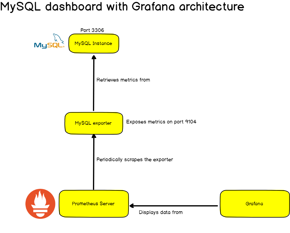
Prometheus is designed to monitor targets. Servers, databases, standalone virtual machines, pretty much everything can be monitored with Prometheus.
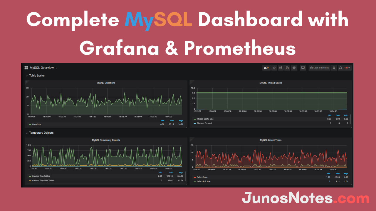
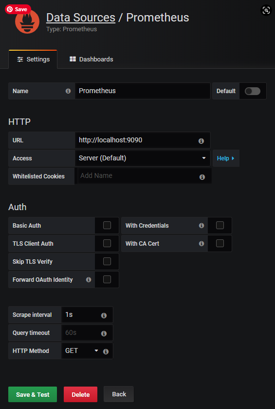
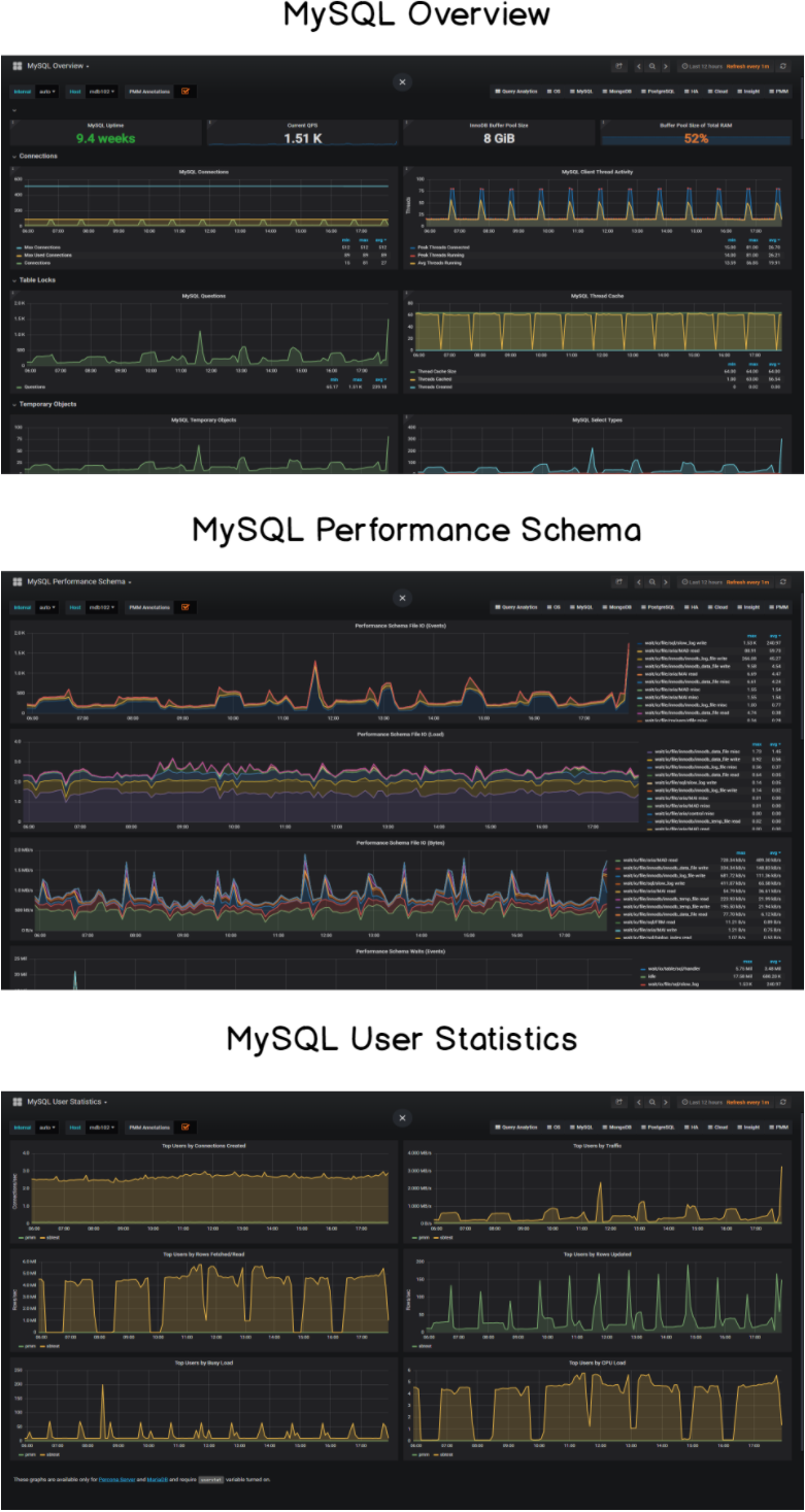
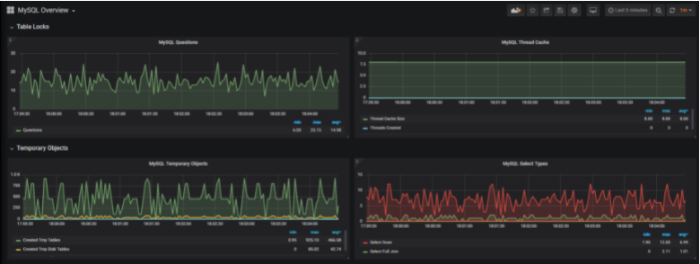
- Complete MySQL dashboard with Grafana & Prometheus | MySQL Database Monitoring using Grafana and Prometheus
- How To Install Prometheus with Docker on Ubuntu 18.04
- Complete Node Exporter Mastery with Prometheus | Monitoring Linux Host Metrics WITH THE NODE EXPORTER
In order to monitor systems, Prometheus will periodically scrap them.
What do we mean by target scraping?
Prometheus expects to retrieve metrics via HTTP calls done to certain endpoints that are defined in the Prometheus configuration.
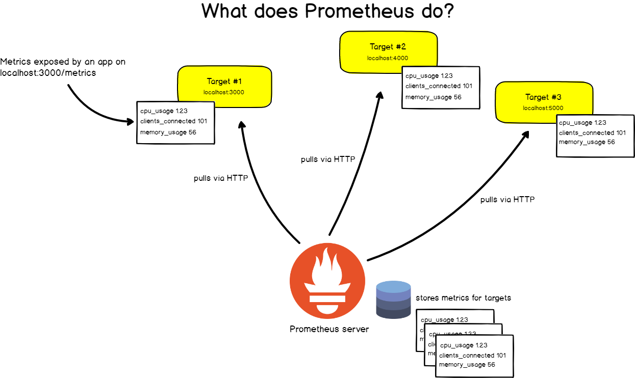
If we take the example of a web application, located at http://localhost:3000 for example, your app will expose metrics as plain text at a certain URL, http://localhost:3000/metrics for example.
From there, on a given scrap interval, Prometheus will pull data from this target.
How does Prometheus work?
As stated before, Prometheus is composed of a wide variety of different components.
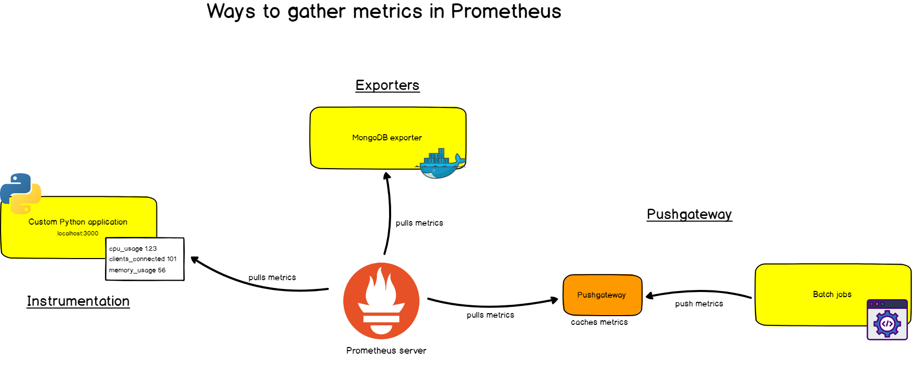
First, you want to be able to extract metrics from your systems. You can do it in very different ways :
- By ‘instrumenting‘ your application, meaning that your application will expose Prometheus compatible metrics on a given URL. Prometheus will define it as a target and scrap it on a given period.
- By using the prebuilt exporters: Prometheus has an entire collection of exporters for existing technologies. You can for example find prebuilt exporters for Linux machine monitoring (node exporter), for very established databases (SQL exporter or MongoDB exporter), and even for HTTP load balancers (such as the HAProxy exporter).
- By using the Pushgateway: sometimes you have applications or jobs that do not expose metrics directly. Those applications are either not designed for it (such as batch jobs for example), or you may have made the choice not to expose those metrics directly via your app.
As you understood it, and if we ignore the rare cases where you might use Pushgateway, Prometheus is a pull-based monitoring system.
What does that even mean? Why did they make it that way?
Pull vs Push
There is a noticeable difference between Prometheus monitoring and other time-series databases: Prometheus actively screens targets in order to retrieve metrics from them.
This is very different from InfluxDB for example, where you would essentially push data directly to it.
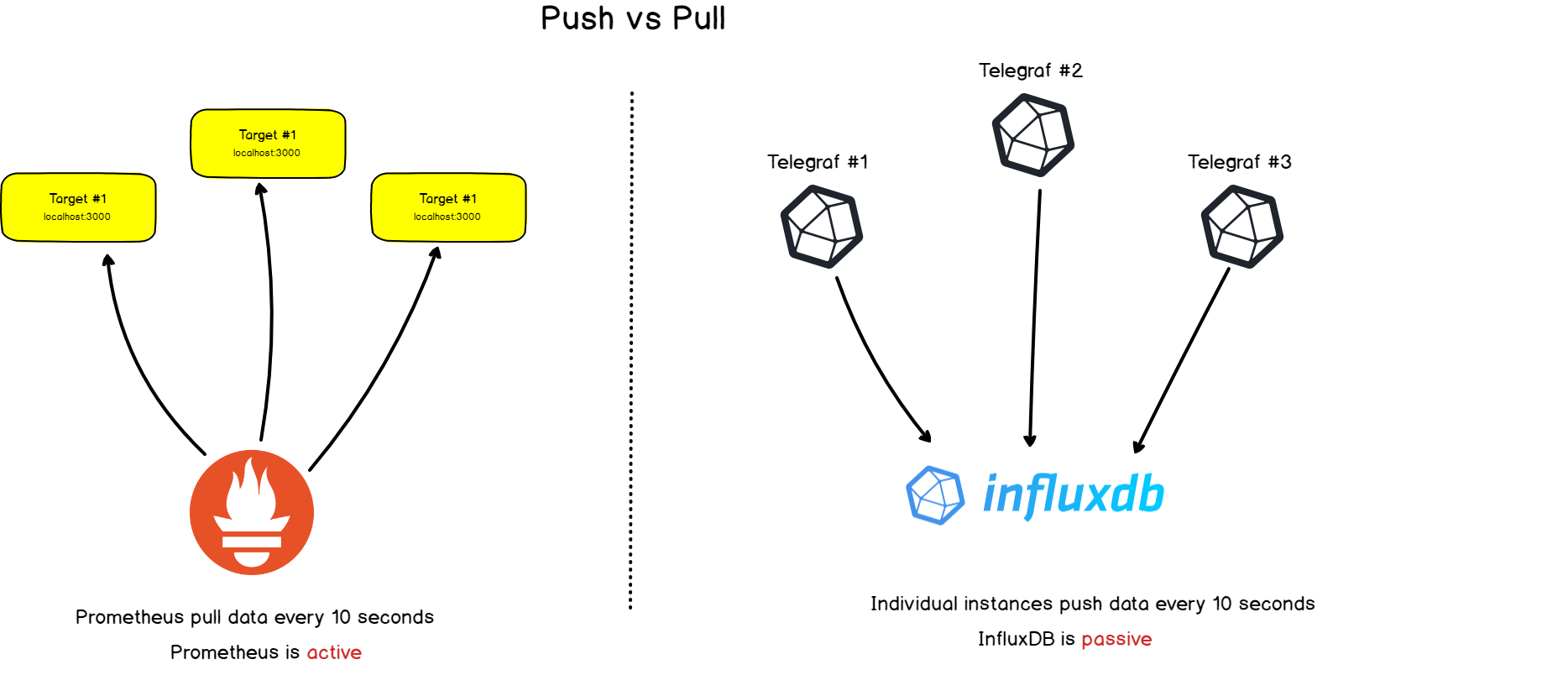
Both approaches have their advantages and inconvenience. From the literature available on the subject, here’s a list of reasons behind this architectural choice:
- Centralized control: if Prometheus initiates queries to its targets, your whole configuration is done on the Prometheus server-side and not on your individual targets.
Prometheus is the one deciding who to scrap and how often you should scrap them.
With a push-based system, you may have the risk of sending too much data towards your server and essentially crash them. A pull-based system enables a rate control with the flexibility of having multiple scrap configurations, thus multiple rates for different targets.
- Prometheus is meant to store aggregated metrics.
This point is actually an addendum to the first part that discussed Prometheus’s role.
Prometheus is not an event-based system and this is very different from other time-series databases. Prometheus is not designed to catch individual and punctual events in time (such as a service outage for example) but it is designed to gather pre-aggregated metrics about your services.
Concretely, you won’t send a 404 error message from your web service along with the message that caused the error, but you will send the fact your service received one 404 error message in the last five minutes.
This is the basic difference between a time series database targeted for aggregated metrics and one designed to gather ‘raw metrics’
Prometheus monitoring rich ecosystem
The main functionality of Prometheus, besides monitoring, is being a time series database.
However, when playing with Time Series Database, you often need to visualize them, analyze them, and have some custom alerting on them.
Here are the tools that compose Prometheus ecosystem to enrich its functionalities :
- Alertmanager: Prometheus pushes alerts to the Alertmanager via custom rules defined in configuration files. From there, you can export them to multiple endpoints such as Pagerduty or Slack.
- Data visualization: Similar to Grafana, you can visualize your time series directly in Prometheus Web UI. You can easily filter and have a concrete overview of what’s happening on your different targets.
- Service discovery: Prometheus can discover your targets dynamically and automatically scrap new targets on demand. This is particularly handy when playing with containers that can change their addresses dynamically depending on demand.
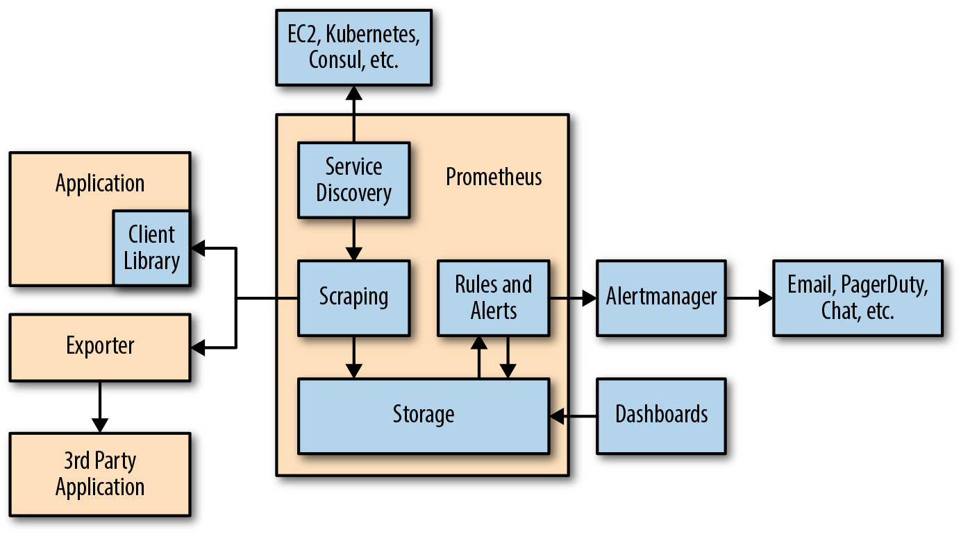
Credits: Oreilly publication
Concepts Explained About Prometheus Monitoring
As we did for InfluxDB, we are going to go through a curated list of all the technical terms behind monitoring with Prometheus.
a – Key-Value Data Model
Before starting with Prometheus tools, it is very important to get a complete understanding of the data model.
Prometheus works with key value pairs. The key describes what you are measuring while the value stores the actual measurement value, as a number.
Remember: Prometheus is not meant to store raw information like plain text as it stores metrics aggregated over time.
The key in this case is called a metric. It could be for example a CPU rate or memory usage.
But what if you wanted to give more details about your metric?
What if my CPU has four cores and I want to have four separate metrics for them?
This is where the concept of labels comes into play. Labels are designed to provide more details to your metrics by appending additional fields to it. You would not simply describe the CPU rate but you would describe the CPU rate for core one located at a certain IP for example.
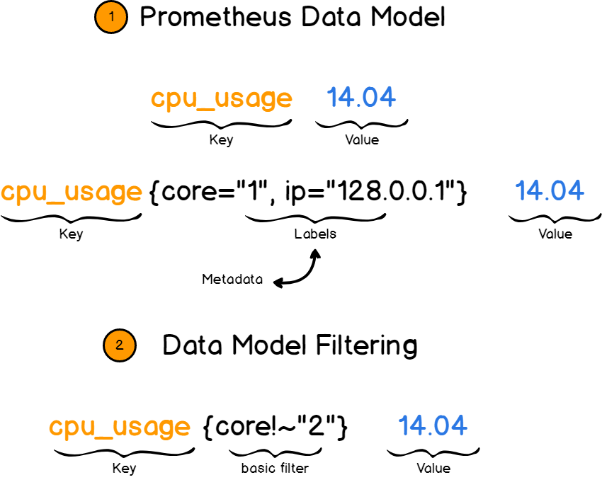
Later on, you would be able to filter metrics based on labels and retrieve exactly what you are looking for.
b – Metric Types
When monitoring a metric, there are essentially four ways you can describe it with Prometheus. I encourage you to follow until the end as there is a little bit of a gotcha with those points.
Counter
Probably the simplest form of the metric type you can use. A counter, as its name describes, counts elements over time.
If for example, you want to count the number of HTTP errors on your servers or the number of visits on your website, you probably want to use a counter for that.
As you would physically imagine it, a counter only goes up or resets.
As a consequence, a counter is not naturally adapted for values that can go down or for negative ones.
A counter is particularly suited to count the number of occurrences of a certain event on a period, i.e the rate at which your metric evolved over time.
Now, what if you wanted to measure the current memory usage at a given time for example?
The memory usage can go down, how can it be measured with Prometheus?
Gauges
Meet gauges!
Gauges are designed to handle values that may decrease over time. Visually, they are like thermomethers: at any given time, if you observe the thermomether, you would be able to see the current temperature value.
But, if gauges can go up and down, accept positive or negative values, aren’t they a superset of counters?
Are counters useless?
This is what I thought when I first met gauges. If they can do anything, let’s use gauges everywhere, right?
Wrong.
Gauges are perfect when you want to monitor the current value of a metric that can decrease over time.
However, and this is the big gotcha of this section: gauges can’t be used when you want to see the evolution of your metrics over time. When using gauges, you may essentially lose the sporadic changes of your metrics over time.
Why? Here’s /u/justinDavidow answer on this.
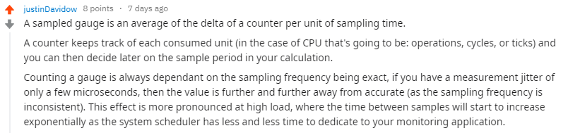
If your system is sending metrics every 5 seconds, and your Prometheus is scraping the target every 15 seconds, you may lose some metrics in the process. If you perform additional computation on those metrics, your results are less and less accurate.
With a counter, every value is aggregated in it. When Prometheus scraps it, it will be aware that a value was sent during a scraping interval.
End of the gotcha!
Histogram
The histogram is a more complex metric type. It provides additional information for your metrics such as the sum of the observations and the count of them.
Values are aggregated in buckets with configurable upper bounds. It means that with histograms you are able to :
- Compute averages: as they represent the fraction of the sum of your values divided by the number of values recorded.
- Compute fractional measurements on your values: this is a very powerful tool as it allows you to know for a given bucket how many values follow given criteria. This is especially interesting when you want to monitor proportions or establish quality indicators.
In a real-world context, I want to be alerted when 20% of my servers respond in more than 300ms or when my servers respond in more than 300ms more than 20% of the time.
As soon as proportions are involved, histograms can and should be used.
Summaries
Summaries are an extension of histograms. Besides also providing the sum and the count of observations, they provide quantiles metrics on sliding windows.
As a reminder, quantiles are ways to divide your probability density into ranges of equal probability.
So, histograms or summaries?
Essentially, the intent is different.
Histograms aggregate values over time, giving a sum and a count function that makes it easy to see the evolution of a given metric.
On the other hand, summaries expose quantiles over sliding windows (i.e continuously evolving over time).
This is particularly handy to get the value that represents 95% of the values recorded over time.
c – Jobs & Instances
With the recent advancements made in distributed architectures and the popularity rise of cloud solutions, you don’t simply have one server standing there, alone.
Servers are replicated and distributed all over the world.
To illustrate this point, let’s take a very classic architecture made of 2 HAProxy servers that redistribute the load on nine backend web servers (No, no, definitely not the Stackoverflow stack..)
In this real-world example, we want to monitor the number of HTTP errors returned by the web servers.
Using Prometheus language, a single web server unit is called an instance. The job would be the fact that you measure the number of HTTP errors for all your instances.
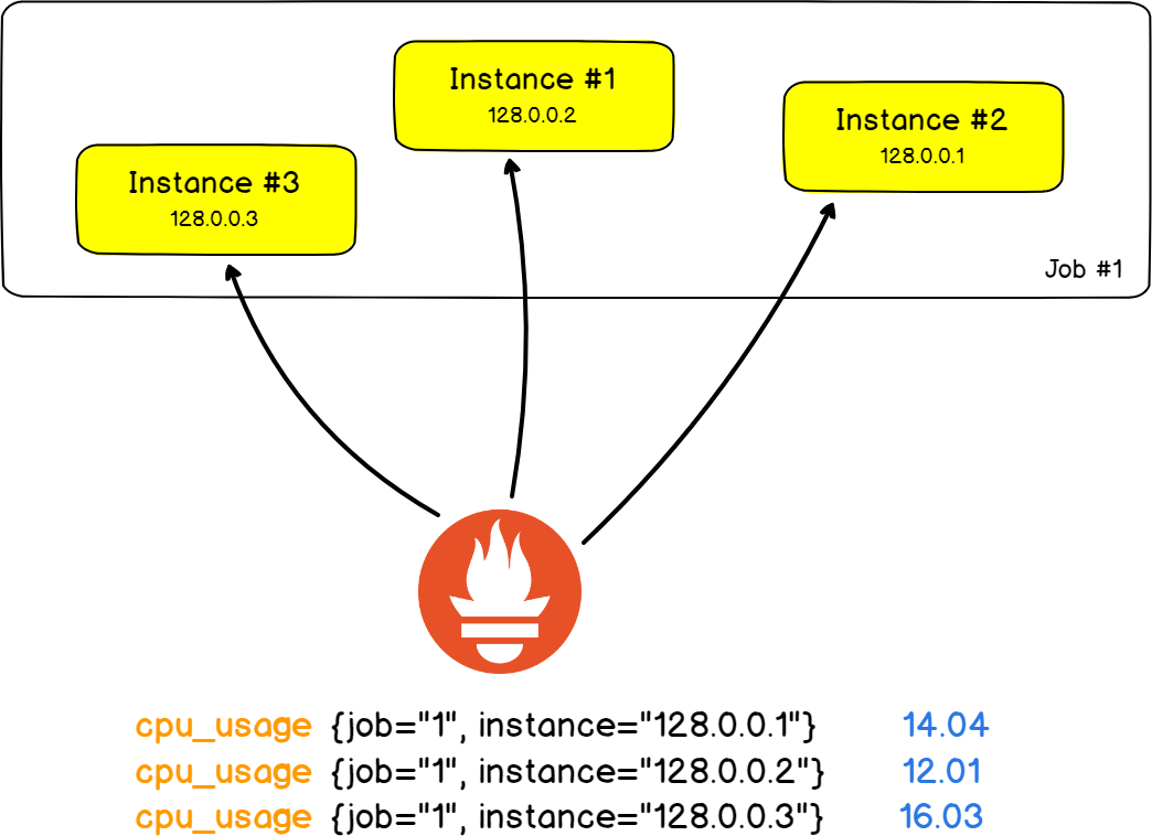
The best part would probably be the fact that jobs and instances become fields in your labels and that you are able to filter your results for a given instance or a given job.
Handy!
d – PromQL
You may already know InfluxQL if you are using InfluxDB based databases. Or maybe you stuck to SQL by using TimescaleDB.
Prometheus also has its own embedded language that facilitates querying and retrieving data from your Prometheus servers: PromQL.
As we saw in the previous sections, data are represented using key value pairs. PromQL is not far from this as it keeps the same syntax and returns results as vectors.
What vectors?
With Prometheus and PromQL, you will be dealing with two kinds of vectors :
- Instant vectors: giving a representation of all the metrics tracked at the most recent timestamp;
- Time ranged vectors: if you want to see the evolution of a metric over time, you can query Prometheus with custom time ranges. The result will be a vector aggregating all the values recorded for the period selected.
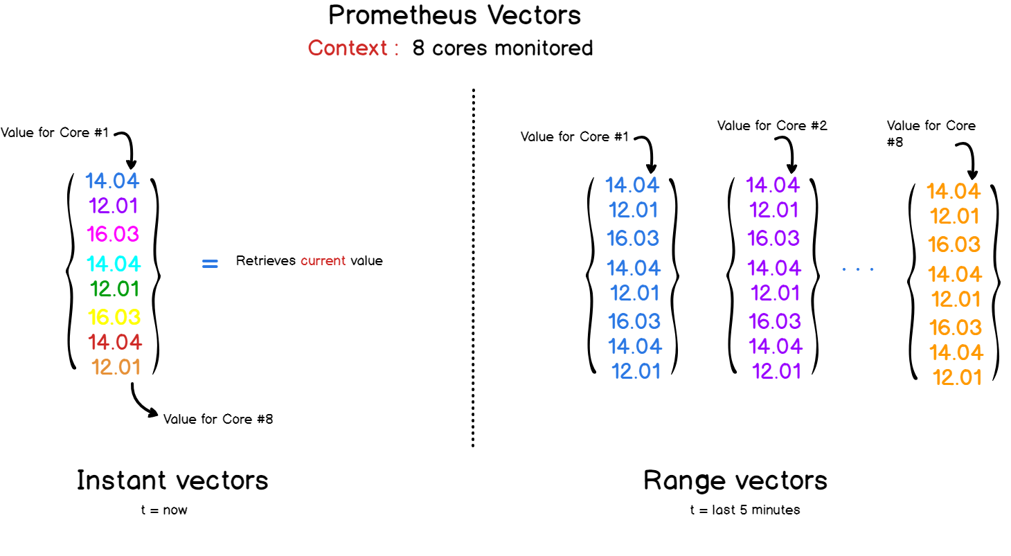
PromQL APIs expose a set of functions that facilitate data manipulation for your queries.
You can sort your values, apply mathematical functions over it (like derivative or exponential functions) and even have some forecasting functions (like the Holt-Winters function).
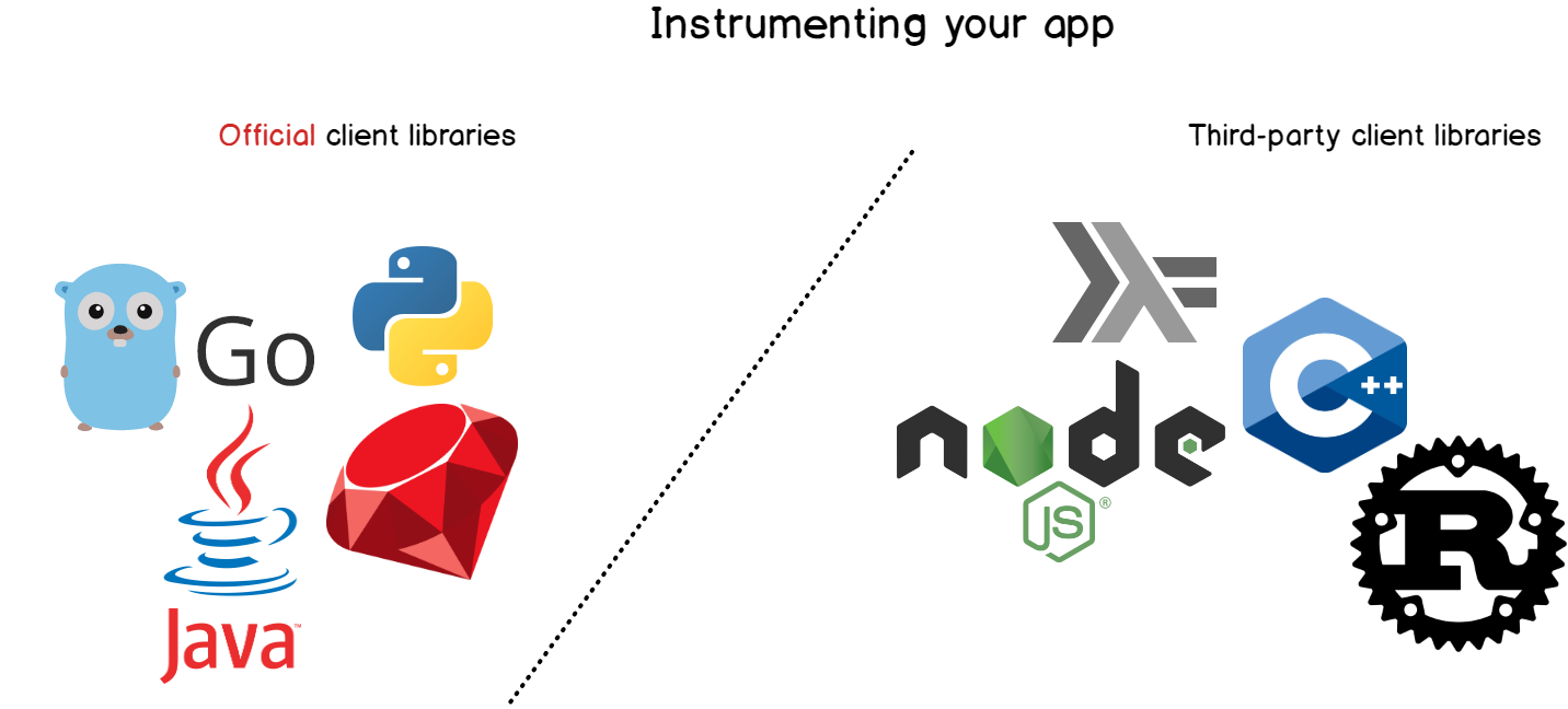
e – Instrumentation
Instrumentation is another big part of Prometheus. Before retrieving data from your applications, you want to instrument them.
Instrumentation in Prometheus terms means adding client libraries to your application in order for them to expose metrics to Prometheus.
Instrumentation can be done for most of the existing programming languages like Python, Java, Ruby, Go, and even Node or C# applications.
While instrumenting, you will essentially create memory objects (like gauges or counters) that you will increment or decrement on the fly.
Later on, you will choose where to expose your metrics. From there, Prometheus will pick them up and store them into its embedded time-series database.
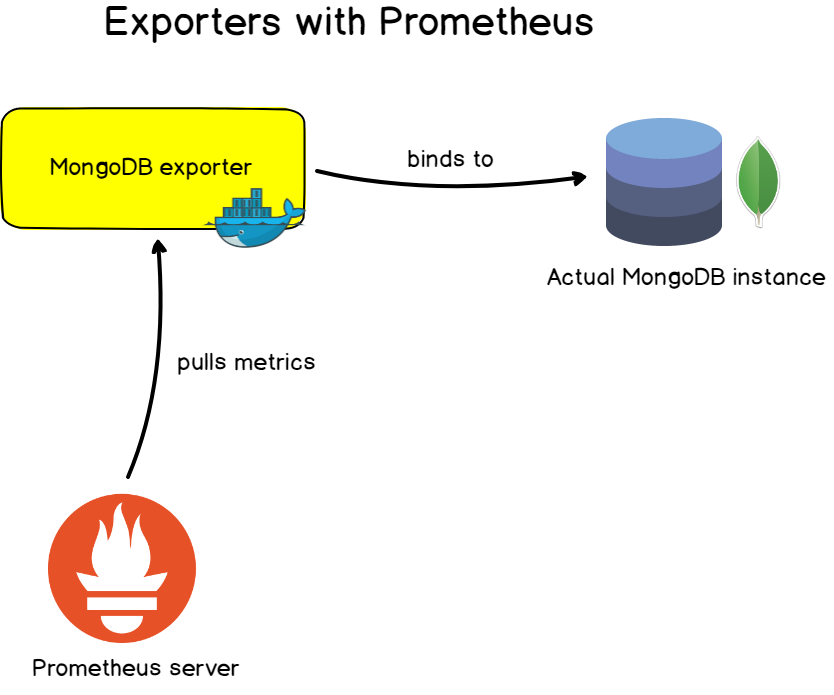
f – Exporters
For custom applications, the instrumentation is very handy at it allows you to customize the metrics exposed and how they are changed over time.
For ‘well-known’ applications, servers, or databases, Prometheus is built with vendors exporters that you can use in order to monitor your targets. This is the main way of monitoring targets with Prometheus.
Those exporters, most of the time exposed as Docker images, are easily configurable to monitor your existing targets. They expose a preset of metrics and often preset dashboards to get your monitoring set in minutes.
Examples of exporters include :
- Database exporters: for MongoDB databases, SQL servers, and MySQL servers.
- HTTP exporters: for HAProxy, Apache, or NGINX servers.
- Unix exporters: you can monitor system performance using built node exporters that expose complete system metrics out of the box.
A word on interoperability
Most time-series databases work hand in hand to promote the interoperability of their respective systems.
Prometheus isn’t the only monitoring system to have a stance on how systems should expose metrics: existing systems such as InfluxDB (via Telegraf), CollectD, StatsD, or Nagios are opiniated on this subject.
However, exporters have been built in order to promote communication between those different systems. Even if Telegraf sends metrics in a format that is different from what Prometheus expects, Telegraf can send metrics to the InfluxDB exporter and will be scraped by Prometheus afterward.
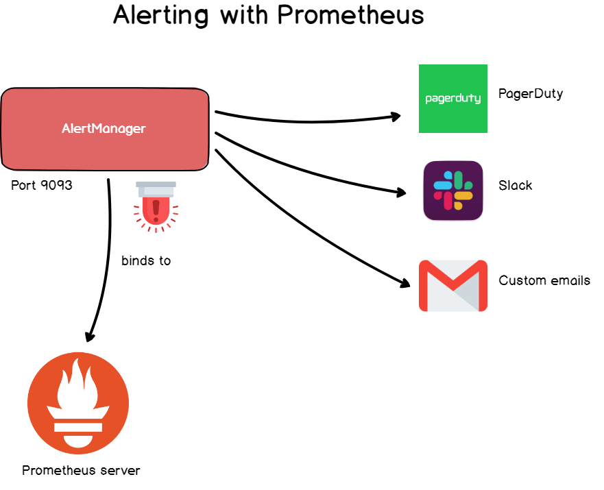
g – Alerts
When dealing with a time-series database, you often want to get feedback from your data and this point is essentially covered by alert managers.
Alerts are a very common thing in Grafana but they are also included in Prometheus via the alert manager.
An alert manager is a standalone tool that binds to Prometheus and runs custom alerts.
Alerts are defined via a configuration file and they define a set of rules on your metrics. If those rules are met in your time series, the alerts are triggered and sent to a predefined destination.
Likewise to what you would find in Grafana, alert destinations include email alerts, Slack webhooks, PagerDuty, and custom HTTP targets.
Prometheus Monitoring Use Cases
As you already know, every definitive guide ends up with a reality check. As I like to say it, technology isn’t an end in itself and should always serve a purpose.
This is what we are going to talk about in this chapter.
a – DevOps Industry
With all the exporters built for systems, databases, and servers, the primary target of Prometheus is clearly targeting the DevOps industry.
As we all know, a lot of vendors are competing for this industry and providing custom solutions for it.
Prometheus is an ideal candidate for DevOps.
The necessary effort to get your instances up and running is very low and every satellite tool can be easily activated and configured on-demand.
Target discovery, via a file exporter, for example, makes it also an ideal solution for stacks that rely heavily on containers and on distributed architectures.
In a world where instances are created as fast as they are destroyed, service discovery is a must-have for every DevOps stack.
b – Healthcare
Nowadays, monitoring solutions are not made only for IT professionals. They are also made to support large industries, providing resilient and scalable architectures for healthcare.
As the demand grows more and more, the IT architectures deployed have to match that demand. Without a reliable way to monitor your entire infrastructure, you may run the risk of having massive outages on your services. Needless to say that those dangers have to be minimized for healthcare solutions.
c – Financial Services
The last example was selected from a conference held by InfoQ discussing using Prometheus for financial institutions.
The talk was presented by Jamie Christian and Alan Strader that showcased how exactly they are using Prometheus to monitor their infrastructure at Northern Trusts. Definitely instructive and worth watching.
Going Further
As I like to believe it, there is a time for theory and a time for practice.
Today, you have been introduced to the fundamentals of Prometheus monitoring, what Prometheus helps you to achieve, its ecosystem, as well as an entire glossary of technical terms, explained.
To begin your Prometheus monitoring journey, start by taking a look at all the exporters that Prometheus offers. Accordingly, install the tools needed, create your first dashboard, and you are ready to go!
If you need some inspiration, I wrote an article on Linux process monitoring with Prometheus and Grafana. It helps setting up the tools as well as getting your first dashboard done.
If you would rather stick to official exporters, here is a complete guide for the node exporter.
I hope you learned something new today.
If there is a subject you want me to describe in a future article, make you leave your idea, it always helps.
Until then, have fun, as always.