How To Setup Telegraf InfluxDB and Grafana on Linux

How To Setup Telegraf InfluxDB and Grafana on Linux | TIG Stack Setup on Linux

The TIG (Telegraf, InfluxDB, and Grafana) stack is apparently the most famous among all existing modern monitoring tools. Also, this stack is very helpful in monitoring a board panel of various datasources like from Operating systems to databases. There are unlimited possibilities and the origin of the TLG stack is very easy to follow.

Today’s tutorial is mainly on How To Setup Telegraf InfluxDB and Grafana on Linux along with that you can also gain proper knowledge about InfluxDB, Telegraf, and Grafana.

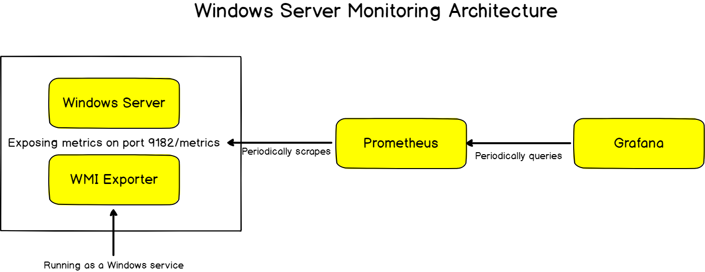
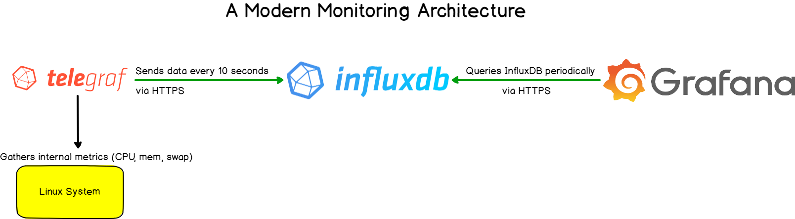
As you can know, Telegraf is a tool that takes responsibility for gathering and aggregating data, like the current CPU usage for instance. InfluxDB will store data, and expose it to Grafana, which is a modern dashboarding solution.

Moreover, we are securing our instances with HTTPS via secure certificates.

modern-monitoring-architecture

Also, it comprises steps for Influx 1.7.x, but I will link to the InfluxDB 2.x setup once it is written.

Prerequisites

If you are following our tutorial to install all these monitoring tools then ensure that you have sudo privileges on the system, otherwise, you won’t be able to install any packages further.

Installing InfluxDB

The complete Installation of InfluxDB can be acquired from this active link. So, make use of it properly and finish your InfluxDB installation.

If you guys looking for the complete guide on How to Install InfluxDB on Windows, then go for it using the available link & start gaining the knowledge.

Later, we are going to learn how to install Telegraf from the below modules:

Installing Telegraf

Telegraf is an agent that collects metrics related to a wide panel of different targets. It can also be used as a tool to processaggregatesplit, or group data.

The whole list of available targets (also called inputs) is available here. In our case, we are going to use InfluxDB as an output.

a – Getting packages on Ubuntu distributions

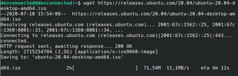
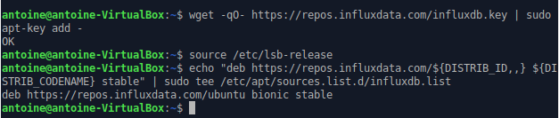
To download packages on Ubuntu 18.04+, run the following commands:

$ wget -qO- https://repos.influxdata.com/influxdb.key | sudo apt-key add -
$ source /etc/lsb-release
$ echo "deb https://repos.influxdata.com/${DISTRIB_ID,,} ${DISTRIB_CODENAME} stable" | sudo tee /etc/apt/sources.list.d/influxdb.list

This is the output that you should see.
install-telegraf-ubuntu

b – Getting packages on Debian distributions.

To install Telegraf on Debian 10+ distributions, run the following commands:

First, update your apt packages and install the apt-transport-https package.

$ sudo apt-get update
$ sudo apt-get install apt-transport-https<

Finally, add the InfluxData keys to your instance.

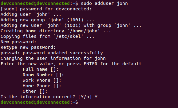
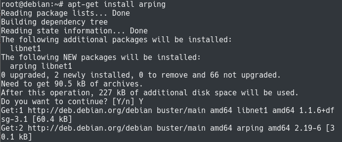
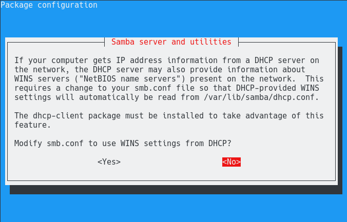
Given your Debian version, you have to choose the corresponding packages.

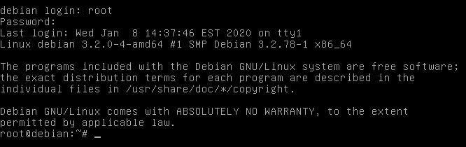
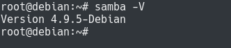
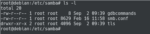
$ cat /etc/debian_version
10.0

get-debian-version

$ wget -qO- https://repos.influxdata.com/influxdb.key | sudo apt-key add -
$ source /etc/os-release


# Debian 7 Wheezy
$ test $VERSION_ID = "7" && echo "deb https://repos.influxdata.com/debian wheezy stable" | sudo tee /etc/apt/sources.list.d/influxdb.list

# Debian 8 Jessie
$ test $VERSION_ID = "8" && echo "deb https://repos.influxdata.com/debian jessie stable" | sudo tee /etc/apt/sources.list.d/influxdb.list

# Debian 9 Stretch
$ test $VERSION_ID = "9" && echo "deb https://repos.influxdata.com/debian stretch stable" | sudo tee /etc/apt/sources.list.d/influxdb.list

# Debian 10 Buster
$ test $VERSION_ID = "10" && echo "deb https://repos.influxdata.com/debian buster stable" | sudo tee /etc/apt/sources.list.d/influxdb.list

debian-10-install

c – Install Telegraf as a service

Now that all the packages are available, it is time for you to install them.

Update your package list and install Telegraf as a service.

$ sudo apt-get update
$ sudo apt-get install telegraf

d – Verify your Telegraf installation

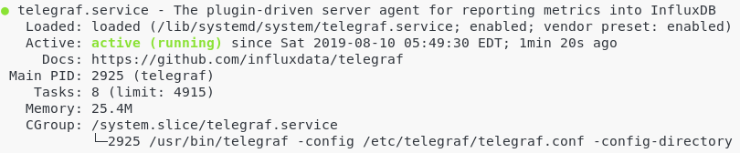
Right now, Telegraf should run as a service on your server.

To verify it, run the following command:

$ sudo systemctl status telegraf

Telegraf should run automatically, but if this is not the case, make sure to start it.

$ sudo systemctl start telegraf

telegraf-running

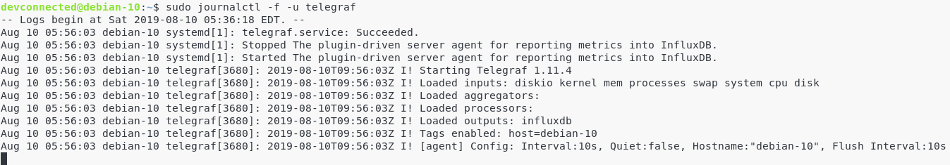
However, even if your service is running, it does not guarantee that it is correctly sending data to InfluxDB.

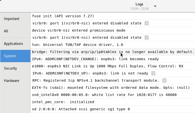
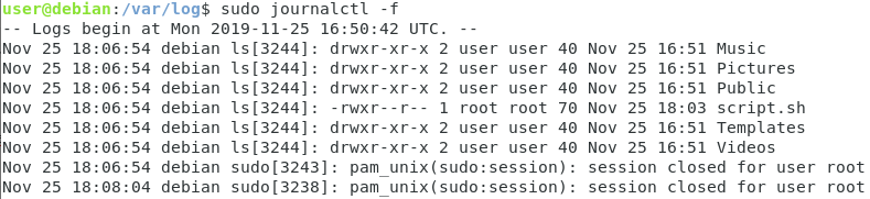
To verify it, check your journal logs.

$ sudo journalctl -f -u telegraf.service

telegraf-running-correctly

If you are having error messages in this section, please refer to the troubleshooting section at the end.

Configure InfluxDB Authentication

In order to have a correct TIG stack setup, we are going to setup InfluxDB authentication for users to be logged in when accessing the InfluxDB server.

a – Create an admin account on your InfluxDB server

Before enabled HTTP authentication, you are going to need an admin account.

To do so, head over to the InfluxDB CLI.

$ influx
Connected to http://localhost:8086 version 1.7.7
InfluxDB shell version: 1.7.7

> CREATE USER admin WITH PASSWORD 'password' WITH ALL PRIVILEGES
> SHOW USERS

user   admin
----   -----
admin  true

b – Create a user account for Telegraf

Now that you have an admin account, create an account for Telegraf

> CREATE USER telegraf WITH PASSWORD 'password' WITH ALL PRIVILEGES
> SHOW USERS

user      admin
----      -----
admin     true
telegraf  true

c – Enable HTTP authentication on your InfluxDB server

HTTP authentication needs to be enabled in the InfluxDB configuration file.

Head over to /etc/influxdb/influxdb.conf and edit the following lines.

[http]
  # Determines whether HTTP endpoint is enabled.
  enabled = true
  
  # The bind address used by the HTTP service.
  bind-address = ":8086"

  # Determines whether user authentication is enabled over HTTP/HTTPS.
  auth-enabled = true

d – Configure HTTP authentication on Telegraf

Now that a user account is created for Telegraf, we are going to make sure that it uses it to write data.

Head over to the configuration file of Telegraf, located at /etc/telegraf/telegraf.conf.

Modify the following lines :

## HTTP Basic Auth
  username = "telegraf"
  password = "password"

Restart the Telegraf service, as well as the InfluxDB service.

$ sudo systemctl restart influxdb
$ sudo systemctl restart telegraf

Again, check that you are not getting any errors when restarting the service.

$ sudo journalctl -f -u telegraf.service

Awesome, our requests are now authenticated.

Time to encrypt them.

Configure HTTPS on InfluxDB

Configuring secure protocols between Telegraf and InfluxDB is a very important step.

You would not want anyone to be able to sniff data you are sending to your InfluxDB server.

If your Telegraf instances are running remotely (on a Raspberry Pi for example), securing data transfer is a mandatory step as there is a very high chance that somebody will be able to read the data you are sending.

a – Create a private key for your InfluxDB server

First, install the gnutls-utils package that might come as gnutls-bin on Debian distributions for example.

$ sudo apt-get install gnutls-utils
(or)
$ sudo apt-get install gnutls-bin

Now that you have the certtool installed, generate a private key for your InfluxDB server.

Head over to the /etc/ssl folder of your Linux distribution and create a new folder for InfluxDB.

$ sudo mkdir influxdb && cd influxdb
$ sudo certtool --generate-privkey --outfile server-key.pem --bits 2048

b – Create a public key for your InfluxDB server

$ sudo certtool --generate-self-signed --load-privkey server-key.prm --outfile server-cert.pem

Great! You now have a key pair for your InfluxDB server.

Do not forget to set permissions for the InfluxDB user and group.

$ sudo chown influxdb:influxdb server-key.pem server-cert.pem

c – Enable HTTPS on your InfluxDB server

Now that your certificates are created, it is time to tweak our InfluxDB configuration file to enable HTTPS.

Head over to /etc/influxdb/influxdb.conf and modify the following lines.

# Determines whether HTTPS is enabled.
  https-enabled = true

# The SSL certificate to use when HTTPS is enabled.
https-certificate = "/etc/ssl/influxdb/server-cert.pem"

# Use a separate private key location.
https-private-key = "/etc/ssl/influxdb/server-key.pem"

Restart the InfluxDB service and make sure that you are not getting any errors.

$ sudo systemctl restart influxdb
$ sudo journalctl -f -u influxdb.service

d – Configure Telegraf for HTTPS

Now that HTTPS is available on the InfluxDB server, it is time for Telegraf to reach InfluxDB via HTTPS.

Head over to /etc/telegraf/telegraf.conf and modify the following lines.

# Configuration for sending metrics to InfluxDB
[[outputs.influxdb]]

# https, not http!
urls = ["https://127.0.0.1:8086"]

## Use TLS but skip chain & host verification
insecure_skip_verify = true
Why are we enabling the insecure_skip_verify parameter?

Because we are using a self-signed certificate.

As a result, the InfluxDB server identity is not certified by a certificate authority. If you want an example of what a full-TLS authentication looks like, make sure to read the guide to centralized logging on Linux.

Restart Telegraf, and again make sure that you are not getting any errors.

$ sudo systemctl restart telegraf
$ sudo journalctl -f -u telegraf.service

Exploring your metrics on InfluxDB

Before installing Grafana and creating our first Telegraf dashboard, let’s have a quick look at how Telegraf aggregates our metrics.

By default, for Linux systems, Telegraf will start gathering related to the performance of your system via plugins named cpu, disk, diskio, kernel, mem, processes, swap, and system.

Names are pretty self-explanatory, those plugins gather some metrics on the CPU usagethe memory usage as well as the current disk read and write IO operations.

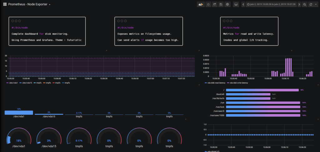
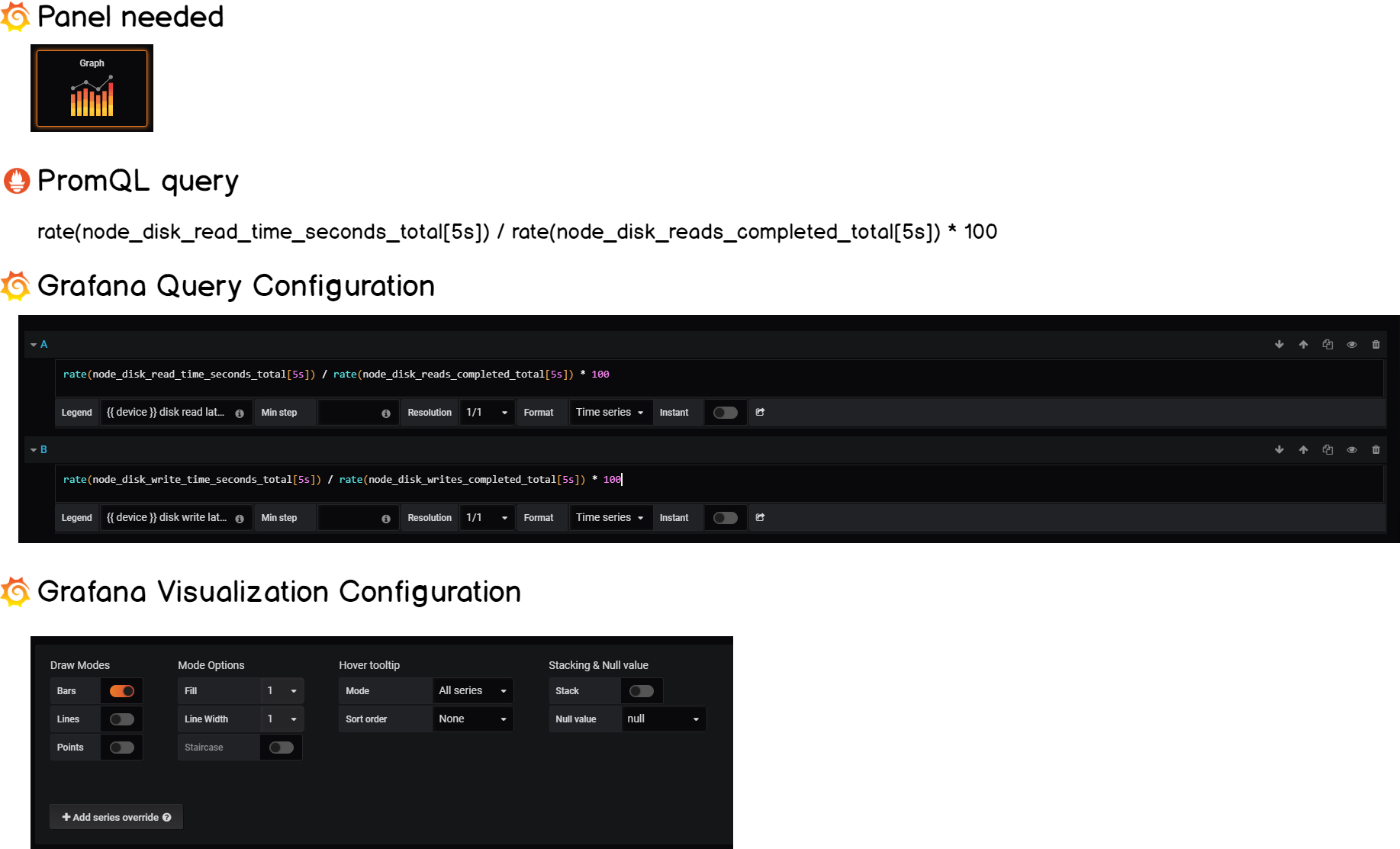
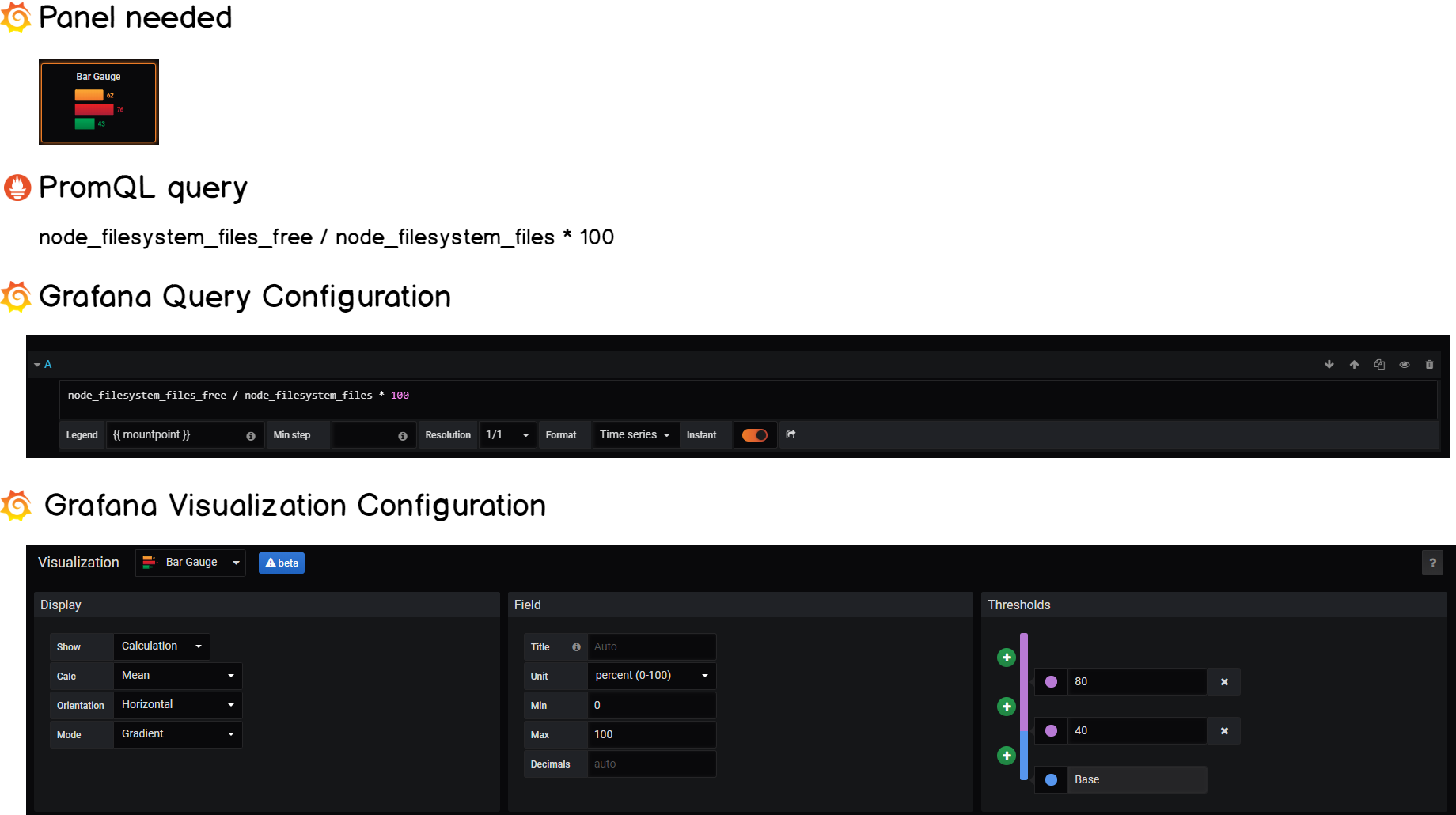
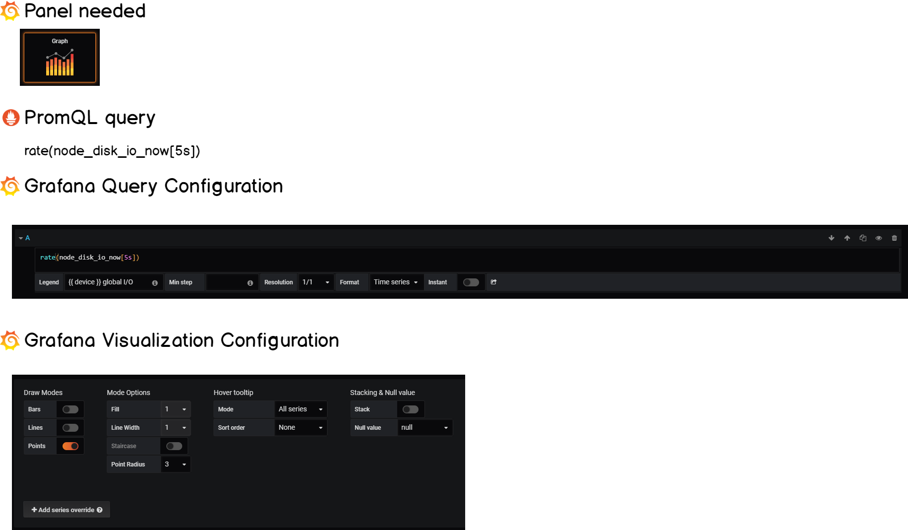
Looking for a tutorial dedicated to Disk I/O? Here’s how to setup Grafana and Prometheus to monitor Disk I/O in real-time.

Let’s have a quick look at one of the measurements.

To do this, use the InfluxDB CLI with the following parameters.

Data is stored in the “telegraf” database, each measurement being named as the name of the input plugin.

$ influx -ssl -unsafeSsl -username 'admin' -password 'password'
Connected to http://localhost:8086 version 1.7.7
InfluxDB shell version: 1.7.7

> USE telegraf
> SELECT * FROM cpu WHERE time > now() - 30s
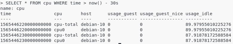
influxdb-query

Great!

Data is correctly being aggregated on the InfluxDB server.

It is time to setup Grafana and builds our first system dashboard.

Installing Grafana

The installation of Grafana has already been covered extensively in our previous tutorials.

You can follow the instructions detailed here in order to install it.

a – Add InfluxDB as a datasource on Grafana

In the left menu, click on the Configuration > Data sources section.

config-datasource

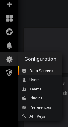
In the next window, click on “Add datasource“.

add-data-source

In the datasource selection panel, choose InfluxDB as a datasource.

influxdb-option

Here is the configuration you have to match to configure InfluxDB on Grafana.

influxdb-config

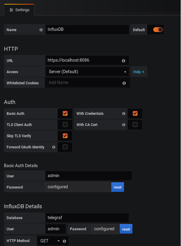
Click on “Save and Test”, and make sure that you are not getting any errors.

data-source-is-working

Getting a 502 Bad Gateway error? Make sure that your URL field is set to HTTPS and not HTTP.

If everything is okay, it is time to create our Telegraf dashboard.

b – Importing a Grafana dashboard

We are not going to create a Grafana dashboard for Telegraf, we are going to use a pre-existing one already developed by the community.

If in the future you want to develop your own dashboard, feel free to do it.

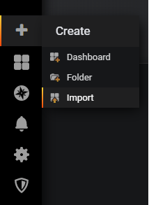
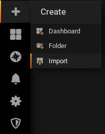
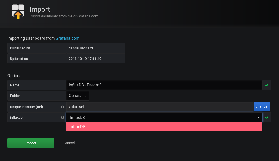
To import a Grafana dashboard, select the Import option in the left menu, under the Plus icon.

import-dashboard (1)

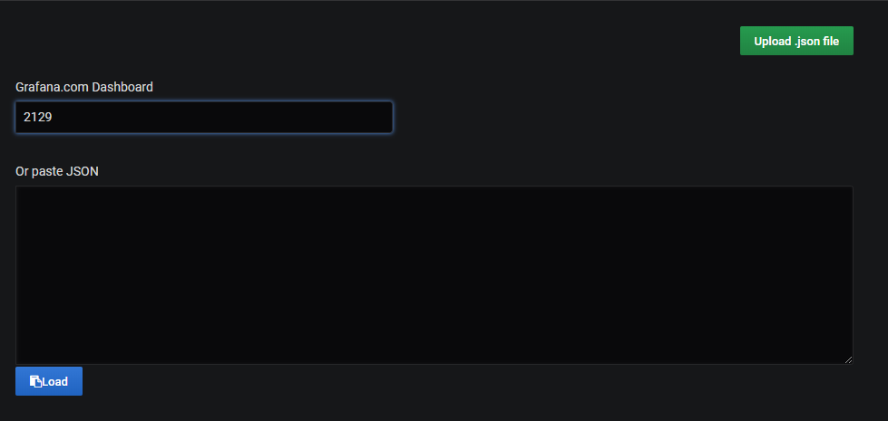
On the next screen, import the dashboard with the 8451 ID.

This is a dashboard created by Gabriel Sagnard that displays system metrics collected by Telegraf.

import-dashboard-23

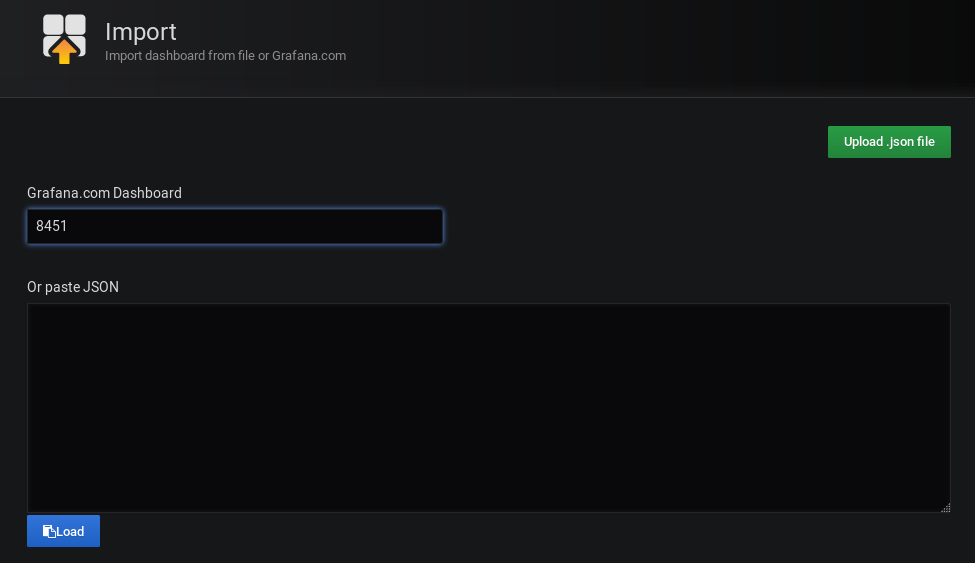
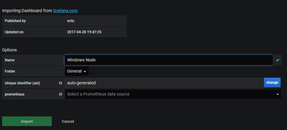
From there, Grafana should automatically try to import this dashboard.

Add the previously configured InfluxDB as the dashboard datasource and click on “Import“.
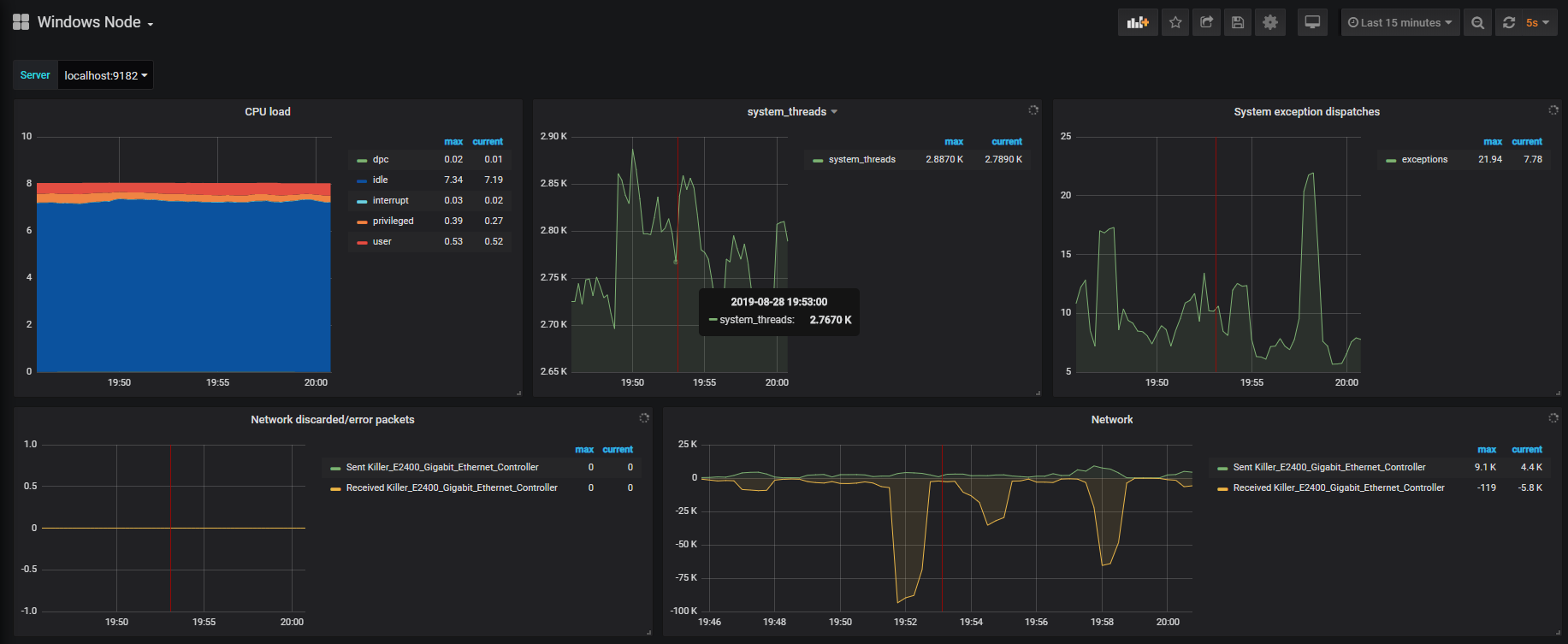
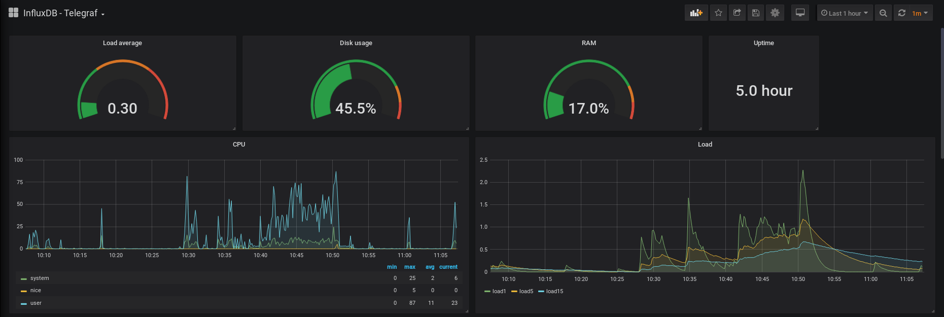
import-dashboard-3

Great!

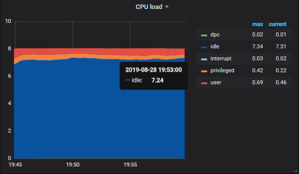
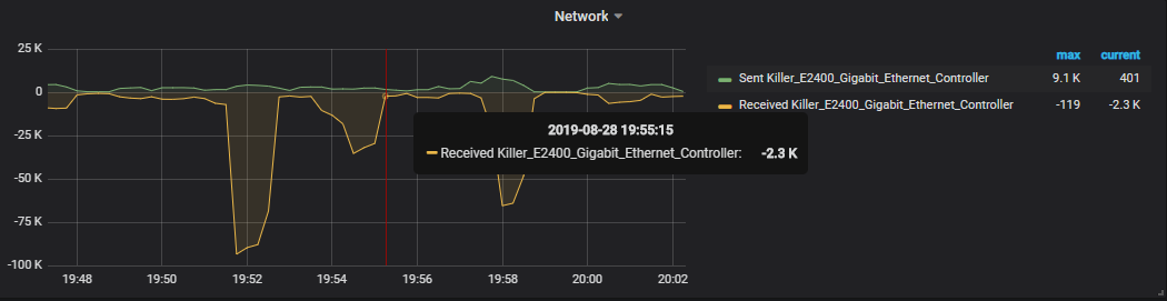
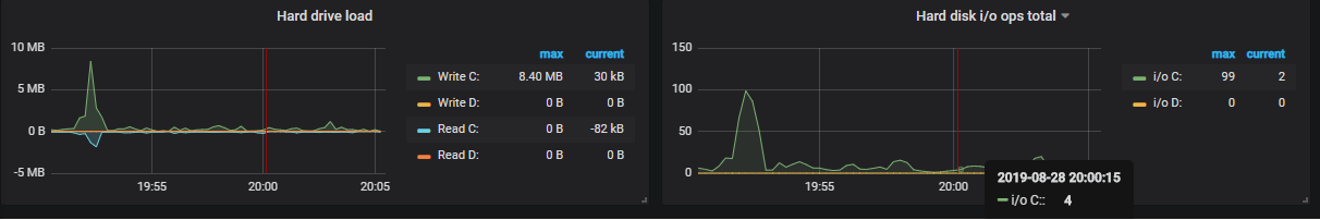
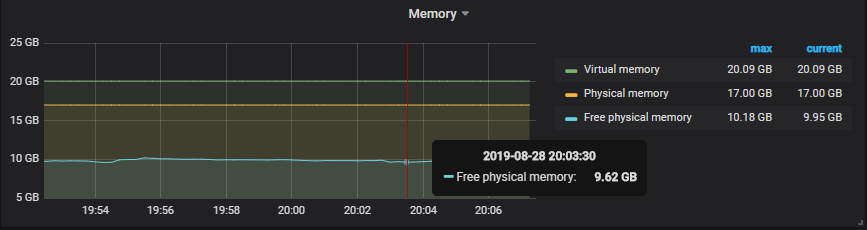
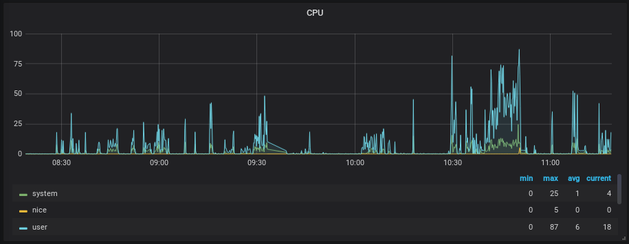
We now have our first Grafana dashboard displaying Telegraf metrics.

This is what you should now see on your screen.

b – Importing a Grafana dashboard final-dashboard

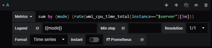
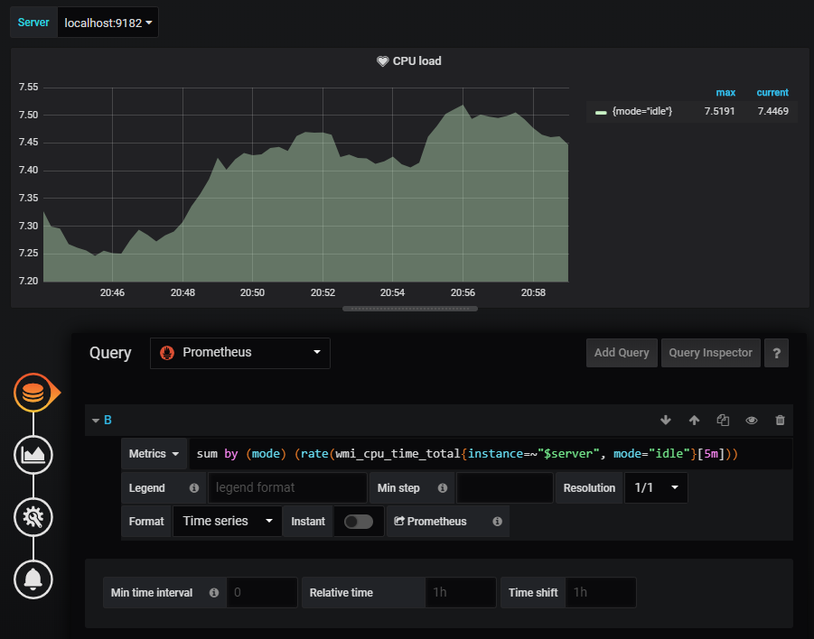
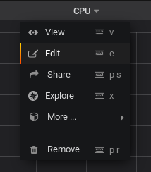
c – Modifying InfluxQL queries in Grafana query explorer

When designing this dashboard, the creator specified the hostname as “Nagisa”, which is obviously different from one host to another (mine is for example named “Debian-10”)

To modify it, head over to the query explorer by hovering the panel title, and clicking on “Edit”.

edit-dashboard

In the “queries” panel, change the host, and the panel should starting displaying data.

changing-host

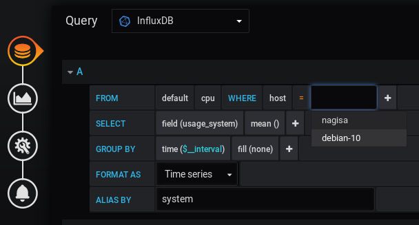
Go back to the dashboard, and this is what you should see.

cpu-dashboard

Conclusion

In this tutorial, you learned how to setup a complete Telegraf, InfluxDB, and Grafana stack on your server.

So where should you go from there?

The first thing would be to connect Telegraf to different inputs, look for existing dashboards in Grafana or design your own ones.

Also, we already made a lot of examples using Grafana and InfluxDB, you could maybe find some inspiration reading those tutorials.

Troubleshooting

  • Error writing to output [influxdb]: could not write any address

error-output-telegraf

Possible solution: make sure that InfluxDB is correctly running on the port 8086.

$ sudo lsof -i -P -n | grep influxdb
influxd   17737        influxdb  128u  IPv6 1177009213      0t0  TCP *:8086 (LISTEN)

If you are having a different port, change your Telegraf configuration to forward metrics to the custom port that your InfluxDB server was assigned.

    • [outputs.influxdb] when writing to [http://localhost:8086] : 401 Unauthorized: authorization failed

Possible solution: make sure that the credentials are correctly set in your Telegraf configuration. Make sure also that you created an account for Telegraf on your InfluxDB server.

    • http: server gave HTTP response to HTTPS client

Possible solution: make sure that you enabled the https-authentication parameter in the InfluxDB configuration file. It is set by default to false.

  • x509: cannot validate certificate for 127.0.0.1 because it does not contain any IP SANs

Possible solution: your TLS verification is set, you need to enable the insecure_skip_verify parameter as the server identity cannot be verified for self-signed certificates.

Windows Server Monitoring using Prometheus and WMI Exporter

Windows Server Monitoring using Prometheus and WMI Exporter | How to Install WMI Exporter in Windows?

Guys who are working as a DevOps engineer or a Site Reliability Engineer should aware of various techniques to monitor their Windows servers. If you are familiar with such tasks then you can easily solve your windows server down issues.

You may get some random doubts whenever your serves go down like Is it due to the high CPU usage on one of the processes? Is the RAM used too much on my Windows server? or Is the server having some memory issues?

To clarify all these queries today we have come up with a new interesting tutorial ie., Windows Server Monitoring using Prometheus and WMI Exporter.

If you are not having an overview of Prometheus Monitoring, check out this Definitive Guide by clicking on the link and start learning about the monitoring of windows servers with Prometheus and WMI Exporter.

Are you ready to monitor your Windows Servers? If yes, then go through these direct links for quick access to the main concept of this tutorial.

What is WMI Exporter?

WMI Exporter is an exporter utilized for windows servers to collects metrics like CPU usage, memory, and Disk usage.

It is open-source which can be installed on Windows servers using the .msi installer

Prerequisites

If you want to follow this tutorial, then you require the following stuff:

  • One Linux server set up
  • Prometheus 2.x installed on your server, including the Prometheus Web UI.
  • Check out your Prometheus version by running the Prometheus -version command. The output comprises your Prometheus version as well as build information.

Windows Server Monitoring Architecture

Before installing the WMI exporter, let’s have a quick look at what our final architecture looks like.

As a reminder, Prometheus is constantly scraping targets.

Targets are nodes that are exposing metrics on a given URL, accessible by Prometheus.

Such targets are equipped with “exporters”: exporters are binaries running on a target and responsible for getting and aggregating metrics about the host itself.

If you were to monitor a Linux system, you would run a “Node Exporter“, which would be responsible for gathering metrics about the CPU usage or the disk I/O currently in use.

For Windows hosts, you are going to use the WMI exporter.

The WMI exporter will run as a Windows service and it will be responsible for gathering metrics about your system.

In short, here is the final architecture that you are going to build.

windows-arch

Installing Prometheus

The complete Prometheus installation for Linux was already covered in one of our previous articles. Check out our Prometheus tutorials main page or else click on this direct link How To Install Prometheus with Docker on Ubuntu 18.04

Ensure to read it extensively to have your Prometheus instance up and running.

To verify it, head over to http://localhost:9090 (9090 being the default Prometheus port).

You should see a Web Interface similar to this one.

If this is the case, it means that your Prometheus installation was successful.

prometheus-homepage

Great!

Now that your Prometheus is running, let’s install the WMI exporter on your Windows Server.

Installing the WMI Exporter

The WMI exporter is an awesome exporter for Windows Servers.

It will export metrics such as CPU usage, memory, and disk I/O usage.

The WMI exporter can also be used to monitor IIS sites and applications, the network interfaces, the services, and even the local temperature!

If you want a complete look at everything that the WMI exporter offers, have a look at all the collectors available.

In order to install the WMI exporter, head over to the WMI releases page on GitHub.

a – Downloading the WMI Exporter MSI

As of August 2019, the latest version of the WMI exporter is 0.8.1.

wmi-exporter-v0.8.1

On the releases page, download the MSI file corresponding to your CPU architecture.

In my case, I am going to download the wmi_exporter-0.8.1-amd64.msi file.

b – Running the WMI installer

When the download is done, simply click on the MSI file and start running the installer.

This is what you should see on your screen.

wmi-exporter-msi

Windows should now start configuring your WMI exporter.
configuring-the-wmi-exporter

You should be prompted with a firewall exception. Make sure to accept it for the WMI exporter to run properly.

The MSI installation should exit without any confirmation box. However, the WMI exporter should now run as a Windows service on your host.

To verify it, head over to the Services panel of Windows (by typing Services in the Windows search menu).

In the Services panel, search for the “WMI exporter” entry in the list. Make sure that your service is running properly.

wmi-exporter-service

c – Observing Windows Server metrics

Now that your exporter is running, it should start exposing metrics on

Open your web browser and navigate to the WMI exporter URL. This is what you should see in your web browser.

Some metrics are very general and exported by all the exporters, but some of the metrics are very specific to your Windows host (like the wmi_cpu_core_frequency_mhz metric for example)

prom-metrics

Great!

Now, Windows Server monitoring is active using the WMI exporter.

If you remember correctly, Prometheus scrapes targets.

As a consequence, we have to configure our Windows Server as a Prometheus target.

This is done in the Prometheus configuration file.

d – Binding Prometheus to the WMI exporter

As you probably saw from your web browser request, the WMI exporter exports a lot of metrics.

As a consequence, there is a chance that the scrape request times out when trying to get the metrics.

This is why we are going to set a high scrape timeout in our configuration file.

If you want to keep a low scrape timeout, make sure to configure the WMI exporter to export fewer metrics (by specifying just a few collectors for example).

Head over to your configuration file (mine is located at /etc/prometheus/prometheus.yml) and edit the following changes to your file.

scrape_configs:
# The job name is added as a label `job=<job_name>` to any timeseries scraped from this config.
  - job_name: 'prometheus'

    # Careful, the scrape timeout has to be lower than the scrape interval.
    scrape_interval: 6s
    scrape_timeout: 5s
    static_configs:
            - targets: ['localhost:9090', 'localhost:9216']

Save your file, and restart your Prometheus service.

$ sudo systemctl restart prometheus
$ sudo systemctl status prometheus

Head back to the Prometheus UI, and select the “Targets” tab to make sure that Prometheus is correctly connected to the WMI exporter.

wmi-target

If you are getting the following error, “context deadline exceeded”, make sure that the scrape timeout is set in your configuration file.

Great! Our Windows Server monitoring is almost ready.

Now it is time for us to start building an awesome Grafana dashboard to monitor our Windows Server.

Building an Awesome Grafana Dashboard

Complete MySQL dashboard with Grafana & Prometheus and MongoDB Monitoring with Grafana & Prometheus are some of our previous guides on Prometheus & Grafana installation. Make sure to configure your Grafana properly before moving to the next section.

If you are looking to install Grafana on Windows, here is another guide for it.

Prometheus should be configured as a Grafana target and accessible through your reverse proxy.

a – Importing a Grafana dashboard

In Grafana, you can either create your own dashboards or you can use pre-existing ones that contributors already crafted for you.

In our case, we are going to use the Windows Node dashboard, accessible via the 2129 ID.

Head over to the main page of Grafana (located at http://localhost:3000 by default), and click on the Import option in the left menu.

import-grafana
In the next window, simply insert the dashboard ID in the corresponding text field.
import-dash-1
From there, Grafana should automatically detect your dashboard as the Windows Node dashboard. This is what you should see.
windows-node-dashboard
Select your Prometheus datasource in the “Prometheus” dropdown, and click on “Import” for the dashboard to be imported.
final-dashboard-2-1

Awesome!

An entire dashboard displaying Windows metrics was created for us in just one click.

As you can see, the dashboard is pretty exhaustive.

You can monitor the current CPU load, but also the number of threads created by the system, and even the number of system exceptions dispatched.

cpu-load

On the second line, you have access to metrics related to network monitoring. You can for example have a look at the number of packets sent versus the number of packets received by your network card.

It can be useful to track anomalies on your network, in case of TCP flood attacks on your servers for example.

network-1

On the third line, you have metrics related to the disk I/O usage on your computer.

Those metrics can be very useful when you are trying to debug applications (for example ASP.NET applications). Using those metrics, you can see if your application consumes too much memory or too much disk.

disk-io-1

Finally, one of the greatest panels has to be memory monitoring. RAM has a very big influence on the overall system performance.

Consequently, it has to be monitored properly, and this is exactly what the fourth line of the dashboard does.

memory-1

That’s an awesome dashboard, but what if we want to be alerted whenever the CPU usage is too high for example?

Wouldn’t it be useful for our DevOps teams to know about it in order to see what’s causing the outage on the machine?

This is what we are going to do in the next section.

Raising alerts in Grafana on high CPU usage

As discussed in the previous section, you want alerts to be raised when the CPU usage is too high.

Grafana is equipped with an alerting system, meaning that whenever a panel raises an alert it will propagate the alert to “notification channels“.

Notification channels are Slack, your internal mailing system of PagerDuty for example.

In this case, we are going to use Slack as it is a pretty common team productivity tool used in companies.

a – Creating a Slack webhook

For those who are not familiar with Slack, you can create webhooks that essentially address for external sources to reach Slack.

As a consequence, Grafana will post the alert to the Webhook address, and it will be displayed in your Slack channel.

To create a Slack webhook, head over to your Slack apps page.

slack-apps-1

Click on the name of your app (“devconnected” here). On the left menu, click on “Incoming Webhooks”.

slack-apps-2

On the next page, simply click on “Add New Webhook to Workspace“.

slack-apps-3

On the next screen, choose where you want your alert messages to be sent. In this case, I will choose the main channel of my Slack account.
slack-apps-4

Click on “Allow”. From there, your Slack Webhook URL should be created.

webhook-URL

b – Set Slack as a Grafana notification channel

Copy the Webhook URL and head over to the Notifications Channels window of Grafana. This option is located in the left menu.

notif-channel

Click on the option, and you should be redirected to the following window.

add-channel

Click on “Add channel”. You should be redirected to the notification channel configuration page.

Copy the following configuration, and change the webhook URL with the one you were provided with in the last step.

slack-config

When your configuration is done, simply click on “Send Test” to send a test notification to your Slack channel.

test-notif

Great! Your notification channel is working properly.

Let’s create a PromQL query to monitor our CPU usage.

c – Building a PromQL query

If you are not familiar with PromQL, there is a section dedicated to this language in my Prometheus monitoring tutorial.

When taking a look at our CPU usage panel, this is the PromQL query used to display the CPU graph.

promQL-1

First, the query splits the results by the mode (idle, user, interrupt, DPC, privileged). Then, the query computes the average CPU usage for a five minutes period, for every single mode.

In the end, the modes are displayed with aggregated sums.

In my case, my CPU has 8 cores, so the overall usage sums up to 8 in the graph.

8-cpus

If I want to be notified when my CPU usage peaks at 50%, you essentially want to trigger an alert when the idle state goes below 4 (as 4 cores are going to be fully used).

To monitor our CPU usage, we are going to use this query

sum by (mode) (rate(wmi_cpu_time_total{instance=~"localhost:9182", mode="idle"}[5m]))

I am not using a template variable here for the instance as they are not supported by Grafana for the moment.

This query is very similar to the one already implemented in the panel, but it specifies that we specifically want to target the “idle” mode of our CPU.

Replace the existing query with the query we just wrote.

This is what you should now have in your dashboard.

cpu-usage-2

Now that your query is all set, let’s build an alert for it.

d – Creating a Grafana alert

In order to create a Grafana alert, click on the bell icon located right under the query panel.

d – Creating a Grafana alert

In the rule panel, you are going to configure the following alert.

Every 10 seconds, Grafana will check if the average CPU usage for the last 10 seconds was below 4 (i.e using more than 50% of our CPU).

If it is the case, an alert will be sent to Slack, otherwise, nothing happens.

rule-1

Finally, right below this rule panel, you are going to configure the Slack notification channel.

notifications-rule

Now let’s try to bump the CPU usage on our instance.

alertalert

As the CPU usage goes below the 4 thresholds, it should set the panel state to “Alerting” (or “Pending” if you specified a “For” option that is too long).

From there, you should receive an alert in Slack.

slack-alert

As you can see, there is even an indication of the CPU usage (73% in this case).

Great! Now our DevOps is aware that there is an issue on this server and they can investigate what’s happening exactly.

Conclusion

As you can see, monitoring Windows servers can easily be done using Prometheus and Grafana.

With this tutorial, you had a quick overview of what’s possible with the WMI exporter. So what’s next?

From there, you can create your own visualizations, your own dashboards, and your own alerts.

Our monitoring section contains a lot of examples of what’s possible and you can definitely take some inspiration from some of the dashboards.

Until then, have fun, as always.

How To Install AutoFS on Linux

Whether you are an experienced system administrator or just a regular user, you have probably already mounted drives on Linux.

Drives can be local to your machine or they can be accessed over the network by using the NFS protocol for example.

If you chose to mount drives permanently, you have probably added them to your fstab file.

Luckily for you, there is a better and more cost effective way of mounting drives : by using the AutoFS utility.

AutoFS is a utility that mount local or remote drives only when they are accessed : if you don’t use them, they will be unmounted automatically.

In this tutorial, you will learn how you can install and configure AutoFS on Linux systems.

Prerequisites

Before starting, it is important for you to have sudo privileges on your host.

To verify it, simply run the “sudo” command with the “-v” option : if you don’t see any options, you are good to go.

$ sudo -v

If you don’t have sudo privileges, you can follow this tutorial for Debian based hosts or this tutorial for CentOS based systems.

Installing AutoFS on Linux

Before installing the AutoFS utility, you need to make sure that your packages are up-to-date with repositories.

$ sudo apt-get update

Now that your system is updated, you can install AutoFS by running the “apt-get install” command with the “autofs” argument.

$ sudo apt-get install autofs

When installing the AutoFS package, the installation process will :

  • Create multiple configuration files in the /etc directory such as : auto.master, auto.net, auto.misc and so on;
  • Will create the AutoFS service in systemd;
  • Add the “automount” entry to your “nsswitch.conf” file and link it to the “files” source

Right after the installation, make sure that the AutoFS service is running with the “systemctl status” command

$ sudo systemctl status autofs

Installing AutoFS on Linux autofs-service

You can also enable the AutoFS service for it to be run at startup

$ sudo systemctl enable autofs

Now that AutoFS is correctly installed on your system, let’s see how you can start creating your first map.

How AutoFS works on Linux

Maps” are a key concept when it comes to AutoFS.

In AutoFS, you are mapping mount points with files (which is called an indirect map) or a mount point with a location or a device.

In its default configuration, AutoFS will start by reading maps defined in the autofs.master file in the /etc directory.

From there, it will start a thread for all the mount points defined in the map files defined in the master file.

How AutoFS works on Linux autofs

Starting a thread does not mean that the mount point is mounted when you first start AutoFS : it will only be mounted when it is accessed.

By default, after five minutes of inactivity, AutoFS will dismount (or unmount) mount points that are not used anymore.

Note : configuration parameters for AutoFS are available in the /etc/autofs.conf

Creating your first auto map file

Now that you have an idea on how AutoFS works, it is time for you to start creating your very first AutoFS map.

In the /etc directory, create a new map file named “auto.example“.

$ sudo touch /etc/auto.example

The goal of this map file will be to mount a NFS share located on one computer on the network.

The NFS share is located at the IP 192.168.178.29/24 on the local network and it exports one drive located at /var/share.

Before trying to automount the NFS share, it is a good practice to try mounting it manually as well as verifying that you can contact the remote server.

$ ping 192.168.178.29

Creating a direct map

The easiest mapping you can create using AutoFS is called a direct map or a direct mapping.

A direct map directly associates one mount point with a location (for example a NFS location)

Creating your first auto map file direct-mapping

As an example, let’s say that you want to mount a NFS share at boot time on the /tmp directory.

To create a direct map, edit your “auto.example” file and append the following content in it :

# Creating a direct map with AutoFS

# <mountpoint>    <options>    <remote_ip>:<location>   

/tmp              -fstype=nfs  192.168.178.29:/var/share

Now, you will need to add the direct map to your “auto.master” file.

To specify that you are referencing a direct map, you need to use the “-” notation

# Content of the auto.master file

/-    auto.example

direct-map

Now that your master file is modified, you can restart the AutoFS service for the changes to be effective.

$ sudo systemctl restart autofs

$ cd /tmp

Congratulations, you should now be able to access your files over NFS via direct mapping.

Creating a direct map tmp-nfs

Creating an indirect mapping

Now that you have discovered direct mappings, let’s see how you can use indirect mappings in order to mount remote location on your filesystem.

Indirect mappings use the same syntax as direct mappings with one small difference : instead of mounting locations directly to the mountpoint, you are mounting it in a location in this mountpoint.

Creating an indirect mapping

To understand it, create a file named “auto.nfs” and paste the following content in it

nfs    -fstype=nfs  192.168.178.29:/var/share

As you can see, the first column changed : in a direct map, you are using the path to the mountpoint (for example /tmp), but with an indirect map you are specifying the key.

The key will represent the directory name located in the mount point directory.

Edit your “auto.master” file and add the following content in it

/tmp   /etc/auto.nfs

Creating an indirect mapping autonfs

Restart your AutoFS service and head over to the “tmp” directory

$ sudo systemctl restart autofs

$ cd /tmp

By default, there won’t be anything displayed if you list the content of this directory : remember, AutoFS will only mount the directories when they are accessed.

In order for AutoFS to mount the directory, navigate to the directory named after the key that you specified in the “auto.nfs” file (called “nfs” in this case)

$ cd nfs

Awesome!

Your mountpoint is now active and you can start browsing your directory.

Mapping distant home directories

Now that you understand a bit more about direct and indirect mappings, you might ask yourself one question : what’s the point of having indirect mapping when you can simply map locations directly?

In order to be useful, indirect maps are meant to be used with wildcard characters.

One major use-case of the AutoFS utility is to be able to mount home directories remotely.

However, as usernames change from one user to another, you won’t be able to have a clean and nice-looking map file, you would have to map every user in a very redundant way.

# Without wildcards, you have very redundant map files

/home/antoine  <ip>:/home/antoine
/home/schkn    <ip>:/home/schkn
/home/devconnected <ip>:/home/devconnected

Luckily for you, there is a syntax that lets your dynamically create directories depending on what’s available on the server.

To illustrate this, create a new file named “auto.home” in your /etc directory and start editing it.

# Content of auto.home

*    <ip>:/home/&

In this case, there are two wilcards and it simply means that all the directories found in the /home directory on the server will be mapped to a directory of the same name on the client.

To illustrate this, let’s pretend that we have a NFS server running on the 192.168.178.29 IP address and that it contains all the home directories for our users.

# Content of auto.home

*   192.168.178.29:/home/&

Save your file and start editing your auto.master file in order to create your indirect mapping

$ sudo nano /etc/auto.master

# Content of auto.master

/home     /etc/auto.home

Save your master file and restart your AutoFS service for the changes to be applied.

$ sudo systemctl restart autofs

Now, you can head over to the /home directory and you should be able to see the directories correctly mounted for the users.

Note : if you see nothing in the directory, remember that you may need to access the directory one time for it to be mounted by AutoFS

Mapping distant home directories home-dir

Mapping and discovering hosts on your network

If you paid attention to the auto.master file, you probably noticed that there is an entry for the /net directory with a value “-hosts“.

The “-hosts” parameter is meant to represent all the entries defined in the /etc/hosts file.

As a reminder, the “hosts” file can be seen as a simple and local DNS resolver that associates a set of IPs with hostnames.

As an example, let’s define an entry for the NFS server into the /etc/hosts file by filling the IP and the hostname of the machine.

Mapping and discovering hosts on your network dns-resolver

First of all, make sure that some directories are exported on the server by running the “showmount” command on the client.

$ sudo showmount -e <server>

Mapping and discovering hosts on your network showmount

Now that you made sure that some directories are exported, head over to your “auto.master” file in /etc and add the following line.

# Content of auto.master

/net   -hosts

Save your file and restart your AutoFS service for the changes to be applied.

$ sudo systemctl restart autofs

That’s it!

Now your NFS share should be accessible in the /net directory under a directory named after your server hostname.

$ cd /net/<server_name>

$ cd /net/<server_ip>
Note : remember that you will need to directly navigate in the directory for it to be mounted. You won’t see it by simply listing the /net directory on the first mount.

Troubleshooting

In some cases, you may have some troubles while setting up AutoFS : when a device is busy or when you are not able to contact a remote host for example.

  • mount/umount : target is busy

As Linux is a multi-user system, you might have some users browsing some locations that you are trying to mount or unmount (using AutoFS or not)

If you want to know who is navigating the folder or who is using a file, you have to use the “lsof” command.

$ lsof +D <directory>
$ lsof <file>

Troubleshooting lsof

Note : the “+D” option is used in order to list who is using the resource recursively.
  • showmount is hanging when configuring host discovery

If you tried configuring host discovery by using the “-hosts” parameter, you might have verified that your remote hosts are accessible using the “showmount” command.

However, in some cases, the “showmount” command simply hangs as it is unable to contact the remote server.

Most of the time, the server firewall is blocking the requests made by the client.

If you have access to the server, you try to inspect the logs in order to see if the firewall (UFW for example) is blocking the requests or not.

firewall-blocking

  • Debugging using the automount utility

On recent distributions, the autofs utility is installed as a systemd service.

As a consequence, you can inspect the autofs logs by using the “journalctl” command.

$ sudo journalctl -u autofs.service

You can also use the “automount” utility in order to debug the auto mounts done by the service.

$ sudo systemctl stop autofs

$ sudo automount -f -v

Conclusion

In this tutorial, you learnt about the AutoFS utility : how it works and the differences between direct and indirect maps.

You also learnt that it can be configured in order to setup host discovery : out of the box, you can connect to all the NFS shares of your local network which is a very powerful tool.

Finally, you have seen how you can create indirect maps in order to automatically create home directories on the fly.

If you are interested in Linux system administration, we have a complete section dedicated to it, so make sure to have a look!

How To Change Root Password on Debian 10

On Linux, the root account is a special user account on Linux that has access to all files, all commands and that can pretty much do anything on a Linux server.

Most of the time, the root account is disabled, meaning that you cannot access it.

For example, if you did not specify any password for root during the installation process, it might be locked by default.

However, you may want to access the root account sometimes to perform specific tasks.

In this tutorial, you are going to learn how you can change the root password on Debian 10 easily.

Prerequisites

To change the root password on Debian 10, you need to have sudo privileges or to have the actual password of the root account.

$ sudo -l

User <user> may run the following commands on host-debian:
    (ALL : ALL) ALL

If this is the case, you should be able to change the root password.

Be careful : changing the root password on Debian 10 will unlock the root account.

Change root password on Debian using passwd

The easiest way to change the root password on Debian 10 is to run the passwd command with no arguments.

$ sudo passwd

Changing password for user root.
New password:
Retype new password:
passwd: all authentication tokens updated successfully.

Alternatively, you can specify the root user account with the passwd command.

$ sudo passwd root
Recommendation : the root account needs a strong password. It should be at least 10 characters, with special characters, uppercase and lowercase letters.

Also, it should not contain any words that are easily found in a dictionary.

In order to connect as root on Debian 10, use the “su” command without any arguments.

$ su -
Password:
[root@localhost ~]#

Change root password on Debian using passwd su

Change root password on Debian using su

Alternatively, if you are not sudo you can still change the root password if you have the actual root password.

First, make sure to switch user to root by running the “su” command without any arguments.

$ su -
Password:
root@host-debian:~#

Now that you are connected as root, simply run the “passwd” command without any arguments.

$ passwd

Changing password for user root.
New password:
Retype new password:
passwd: all authentication tokens updated successfully.

You can now leave the root account by pressing “Ctrl +D”, you will be redirected your main user account.

Change root password on Debian using su-root

Change root password using single user mode

Another way of changing the root password on Debian 10 is to boot your host in single user mode.

If you are not sure how you can boot a Debian host in single user mode, you can read this tutorial that we wrote on the subject.

Change root password using single user mode root-account

Now that you are logged as root, you can run the “passwd” command in order to change the root password easily.

# passwd

Changing password for user root.
New password:
Retype new password:
passwd: all authentication tokens updated successfully.

Congratulations, you successfully changed the root password on Debian 10!

You can now simply restart your host and start playing with the root account.

Conclusion

In this quick tutorial, you learnt how you can change the root password on Debian 10 : by using the passwd command or by connecting as root and changing your password.

You also learnt that changing the root password can be done by booting your host in single user mode and running the passwd command.

Using the root account can also be quite useful if you plan on adding or deleting users on Debian 10.

If you are interested in Linux system administration, we have a complete section dedicated to it on the website, so make sure to check it out.

How To Install and Configure Ubuntu 20.04 with GNOME

This tutorial provides step by step instructions on how to install Ubuntu 20.04 with a GNOME environment.

As announced on the Ubuntu official website, Canonical has just released a brand new version of Ubuntu on the 23th of April 2020.

Named Focal Fossa (or 20.04), this version of Ubuntu is a long term support version offering the following new features :

  • The GNOME (v3.36) environment is available by default when installing Ubuntu 20.04;
  • Ubuntu 20.04 uses the v5.4 of the Linux kernel : as a reminder, it adds some interesting memory management improvements as well as compatibility with many different hardware devices;
  • Ubuntu toolchain has been upgraded : it now uses Python 3.8.2, OpenJDK 11 (or JavaSE 11), GCC 9.3 and recent versions of NGINX and Apache;
  • Ubuntu desktop environment has seen some improvements and now looks more recent and modern;
  • Improvements have been made on the ZFS filesystem such as native encryption, improved device removal and pool TRIM.

Now that you have a complete idea of the new features of Ubuntu 20.04, let’s see how you can install Ubuntu easily on your computer or server.

Here are the steps to install Ubuntu 20.04.

Create a Bootable Ubuntu 20.04 on Linux

Unless you are working on a virtualized environment (such as VirtualBox), you will need to create a bootable USB stick in order to start the installation.

As a quick reminder, if you are working on Windows, you will have to use Rufus but the steps are essentially the same.

The Ubuntu 20.04 ISO file is available on the official Ubuntu website.

When visiting the website, you essentially have two options :

  • Download an ISO file containing a desktop environment: this is suited for personal computers as well as system administrators not very familiar with the shell environment.
  • Download an ISO file for server administration: you may need to choose this version if you don’t need the desktop environment and rather have features such as an SSH server installed by default.

Create a Bootable Ubuntu 20.04 on Linux

For this tutorial, we are going to use the ISO file containing a desktop environment.

First of all, make sure to plug the USB stick where you want the ISO file to be stored : the ISO file is about 2.5 GBs in size, so make to choose a large enough USB stick.

Plug the USB stick in the USB port

When inserting the USB stick, your distribution should automatically detect the new device.

Plug the USB stick in the USB port insert-usb-stick

You can also check that your device was correctly mounted by running the following command

$ df

Plug the USB stick in the USB port df-command

In this case, the USB stick is linked to the “sdc” filesystem and mounted on the “/home/devconnected/usb” mountpoint.

If you are not very familiar with filesystems and partitions, make sure to read our guides on mounting filesystems.

If you have any doubts, you can also use the “lsblk” command in order to list all block devices available on your computer.

$ lsblk

Plug the USB stick in the USB port lsblk-command

Download Ubuntu 20.04 ISO file

In order to download the ISO file, you have two options : you can either download it directly from the website provided before or use the wget command in order to download the file.

As a reminder, we are going to install the image containing the desktop environment.

In order to download it, execute the “wget” command followed by the link to the ISO file.

$ wget https://releases.ubuntu.com/20.04/ubuntu-20.04-desktop-amd64.iso

Download Ubuntu 20.04 ISO file wget-ubuntu

After a while, the ISO file should be downloaded on your machine.

Copy the image to your USB drive

Now that the ISO is downloaded, it is time to copy it to your USB drive.

$ sudo dd bs=4M if=ubuntu-20.04-desktop-amd64.iso of=/dev/sdc && sync

Boot on the USB drive

Now that your USB stick is ready, you are ready to boot on it.

Depending on the BIOS you are using, you may need to press one of the following keys to escape the normal boot : ESC, F1, F2 or F8.

Install Ubuntu 20.04 from your USB drive

Now that you booted directly from your USB drive, you should see the following screen.

Ubuntu will simply start to check files and their integrity to make sure that you have the correct ISO version.

Install Ubuntu 20.04 from your USB drive-ubuntu-check-disk

When this step is done, you will be prompted with this window : you can either try Ubuntu or install Ubuntu.

In our case, we are going to install Ubuntu.

2-install-ubuntu

Follow Ubuntu installation steps

On the next screen, you are immediately asked to choose a keyboard layout for your computer.

For the example, we are going to choose “English (US) > English(US)”, however feel free to choose the layout that you feel comfortable with.

Follow Ubuntu installation steps-select-language

When clicking on “Continue“, you are asked the type of installation that you want.

4-updates-and-other-software

As we are targeting a rather minimal installation of Ubuntu, we are not going to install the third-party software suggested. We can install them later on when needed.

Stick with the defaults and click on “Continue“.

5-installation-type

Next, you are asked for the partitioning that you want to perform on your instance.

Usually, you can stay with an automatic partitioning (which is essentially “Erase disk and install Ubuntu“).

If you are an advanced system administrator, and if you want to have your own partitioning, you can go for the other option.

However, even if you are going for an automatic partitioning, make sure to have LVM setup from the beginning.

6-use-lvm

Also, if you are not very comfortable with LVM and dynamic volume management, make sure to check our advanced guide on LVM.

Disk encryption will not be used, however if you need this security, make sure to check the encryption box.

Now that everything is ready, you can click on “Install Now” at the bottom of the previous window.

7-install-ubuntu-now

A confirmation window will open asking if you are sure with all the changes that are going to be performed. Read carefully this window as you won’t be able to go back after clicking on “Continue“.

Essentially, the installation wizard will create one partition (named sda) on your computer and it is going to create two volume groups : one for your root filesystem and one for the swap partition.

Click on “Continue” when you have carefully read the modifications.

8-write-changes-to-disk

On the next screen, choose your location on the map by clicking directly on it and click on “Continue“.

9-location

Finally, you are going to create a user for your instance, make sure to choose a name, a computer name (in order to identify it over the network) as well as a secure password.

If you are working on a local network, make sure to choose a computer instance name that is unique, otherwise you might create conflicts related to DNS.
10-create-user
From there the installation will start.
11-install-ubuntu

Reboot your system on installation complete

When the installation is done, you will be prompted with a window asking you to restart now.

Click on “Restart now” and wait for the system to start booting up again.

12-restart-now

Boot in your new Ubuntu image

Now that the system is started, the user you created in the installation process is automatically selected.

13-boot-ubuntu

Use the credentials specified before and log in into your newly created account.

Once you are logged in, pretty much like in the CentOS installation, you will be asked to connect your online accounts (meaning email and social accounts).

14-connect-online-accounts

For this tutorial, we are not going to connect any accounts, but feel free to do it if you want to.

Livepatch setup

Next, you will be asked if you want to install Livepatch. In short, Livepatch is used to install critical features that would usually require a system reboot.

In production environments, this is a crucial feature as your server might be the host for websites or applications that cannot be easily interrupted.

To install Livepatch, simply click on “Set up Livepatch” in the initialization wizard.

15-setup-livepatch

You will be asked to provide your credentials in order to complete this step.

16-authentication-required

Also, you will be asked to have an Ubuntu account in order to setup Livepatch. If this is not the case, make sure to create a Canonical account if you don’t have one already.

17-sign-in-register

In this case, we already have a Ubuntu account, so we are simply going to connect to it.

When this is done, Livepatch will be enabled and active on your system.

20-livepatch-enabled

Awesome, you can click on “Next“.

Complete final installation steps

You are almost at the end of the process.

Then, you are asked if you want to send statistics and computer information directly to Canonical.

For this step, you can choose if you want to send information or not, but for the tutorial, we are going to choose not to do it.

Click on “Next“.

21-help-improve-ubuntu

Again, you are asked if you want applications to have your geolocation. I would recommend to have this option desactivated for now.

If an application needs your geolocation, you will be prompted with it anyway. As stated, “privacy controls can be changed at any time from the “Settings” application.”

22-privacy-settings

Ready to go!

23-ready-to-go

You have successfully completed the Ubuntu 20.04 installation, and you will be able to have all those amazing tools via the “Software” application.

Going Further with Ubuntu 20.04

Now that your server is completely installed, you are ready to create your users and install software that will be needed throughout your Ubuntu journey.

Update your Ubuntu server

First of all, after installing your server (especially if you installed Livepatch in previous steps) you will be prompted with some basic software update.

24-software-update
Simply click on “Install” and wait for the updates to be completely installed.

25-software-update

At the end of the installation, you will be required to restart your server.

If you don’t have this option available, note that you can install update manually by using the APT package manager.

# Updates cache with newly available software
$ sudo apt-get update

# Applies updates downloaded with the previous command
$ sudo apt-get upgrade

Adding your first user

In order to add your first user to your Ubuntu 20.04 server, use the following command

$ sudo adduser <user>
$ sudo passwd <user>

Adding your first user add-user

Adding a user to administrators

In order to add a new user to administrators, use the following command

$ sudo usermod -aG sudo <user>

Adding a user to administrators-add-user-sudo

Conclusion

In this tutorial, you learnt how you can easily install the most recent Ubuntu version : Focal Fossa or Ubuntu 20.04.

This tutorial covers the very first steps of server creation, however you might want to set up a SSH server or install reverse proxies on your server. Those aspects will be covered in our upcoming tutorials.

Until then, we recommend that you familiarize yourself with your new distribution, more specifically with the software installer that contains all the useful software.

Arping Command on Linux Explained

As a network administrator, you are probably already very familiar with the ARP protocol.

ARP is commonly used by layer two devices in order to discover as well as communicating with each other easily.

When you are dealing with a small office network, you might be tempted to ping hosts in order to verify that they are available.

If you are using the ICMP protocol, you might be aware that you are actually performing ARP requests in order to probe devices on your network.

If you are looking for a more straightforward way to create ARP pings, you might be interested in the arping command.

In this tutorial, we are going to focus on the arping command : how to install it and how to use it effectively.

Prerequisites

In order to install the arping command on your system, you will obviously need sudo privileges on your server.

In order to check if you are sudo or not, you can simply execute the following command

$ groups

user sudo

If this is not the case, you can read our guide on getting sudo privileges for Debian or CentOS hosts.

In order to install the arping command on your server, execute the “apt-get install” command and specify the “arping” package.

$ sudo apt-get install arping

Installing arping on Linux arping

Now that the command is installed, you can execute the “arping” command in order to check the current version used.

$ arping -v

ARPing 2.19, by Thomas Habets <thomas@habets.se>

Great!

The arping command is now installed on your server.

By default, the arping command is going to send an ARP (or ICMP) request every second, but it can obviously be configured.

Using arping to discover hosts

First of all, as any device communicating over Ethernet, your device has an internal ARP table used to communicate over the network.

In order to see your current ARP entries, you can simply execute the “arp” command with the “-a” option for all devices.

$ arp -a

When using the ARP command, you are presented with a list of hostnames, followed by IPs and MAC addresses.

Using arping to discover hosts arp-table

In this case, I am presented with the only entry in my ARP table : a router accessible via the 192.168.178.1 IP address.

However, I might be interested in finding other hosts on my local network : to achieve that, you are going to use the arping command.

Pinging hosts using IP addresses

In order to ping hosts over your network, you can simply use the “arping” command and specify the IP address to be pinged.

Additionally, you can specify the number of pings to be sent using the “-c” option for “count”.

$ arping -c 2 <ip_address>
Note : if you are not sure about the way of finding your IP address on Linux, we have a complete guide on the subject.

For example, using the “192.168.178.27” IP address over your local network, you would execute the following command

Pinging hosts using IP addresses arping-example

As you can see, if you are getting response pings, you are presented with the MAC address of the corresponding device.

Note that using the arping command will not automatically update your ARP table : you would have to use a command such as ping in order to update it.

$ arp -a

Pinging hosts using IP addresses arp-update

Awesome, you successfully used the arping command in order to issue ARP requests over the network!

ARP timeouts using arping

If the arping command is not able to resolve the IP address of the target defined, you will get an ARP timeout.

As an example, executing an ARP request on an unknown host would give you the following output

$ arping -c 5 <ip_address>

ARP timeouts using arping-timeout

As you can see, in some cases, you will be presented with a warning if you don’t specify any network interface.

This is quite normal because the arping command expects a network interface to be specified.

If you were to deal with a router, or if you chose to install your Linux server as a router, two network interface cards can be installed in order to route to two different networks.

If this is the case, the arping needs to know the network interface it needs to use in order to send the ARP ping.

As you can see, the arping command will try to “guess” the network interface if it is not provided with one.

Specifying the network interface

If you have multiple network interfaces on your server, the arping won’t be able to “guess” the network interface card to be used.

As a consequence, you might get an error message stating that the arping was not able to guess the correct one.

Specifying the network interface suitable-device-guess

In order to specify the network interface to be used, you will have to use the “-I” option followed by the name of the network interface.

If you need some help on how to enumerate network interfaces, you can use this guide on finding your IP address on Linux.

$ arping -I <interface_name> <ip_address>

If our interface is named “enp0s3”, the command would be the following one :

$ arping -I enp0s3 192.168.178.22

Specifying the network interface arping-network-interface

Awesome, you have pinged your distant server and you have specified the network interface to be used!

Sending ARP pings from Source MAC

In some cases, you may want to specify the source MAC address you are sending packets from.

In order to achieve that, you need to execute the “arping” command with the “-s” option for “source” followed by the MAC address you want to ping.

$ arping -c 2 -s 00:60:70:12:34:56 <ip_address>

In this case, you have two possibilities :

  • You are the owner of the MAC address and you can simply use the “-s” option.
  • You are not the owner of the MAC address and you are trying to spoof the MAC address. In this case, you need to use the promiscuous mode. As a short reminder, the promiscuous mode is set to transmit all frames received by the NIC rather than the ones it was meant to receive.

In order to enable the promiscuous mode with the “arping” command, you need to use the “-p” option.

Using the options we used previously, this would lead us to the following command.

$ arping -c 2 -s 00:60:70:12:34:56 -p <ip_address>

Conclusion

In this tutorial, you learnt how you can easily use the arping in order to ping IP addresses on your local network.

Using arping, you are able to populate your local ARP cache with the matching MAC address.

You also learnt that you are able to “spoof” your MAC address by using the promiscuous mode.

If you are interested in Linux System Administration, we have a complete section dedicated to it on the website, so make sure to check it out!

Monitoring Disk I/O on Linux with the Node Exporter

Monitoring disk I/O on a Linux system is crucial for every system administrator.

When performing basic system troubleshooting, you want to have a complete overview of every single metric on your system : CPU, memory but more importantly a great view over the disk I/O usage.

In our previous tutorial, we built a complete Grafana dashboard in order to monitor CPU and memory usages.

In this tutorial, we are going to build another dashboard that monitors the disk I/O usage on our Linux system, as well as filesystems and even inodes usage.

We are going to use Prometheus to track those metrics, but we will see that it is not the only way to do it on a Linux system.

This tutorial is split into three parts, each providing a step towards a complete understanding of our subject.

  • First, we will see how disk I/O monitoring can be done on a Linux system, from the filesystem itself (yes metrics are natively on your machine!) or from external tools such as iotop or iostat;
  • Then, we will see how Prometheus can help us monitoring our disk usage with the Node exporter. We are going to set up the tools, set them as services and run them;
  • Finally, we are going to setup a quick Grafana dashboard in order to monitor the metrics we gathered before.
Ready?

Lesson 1 – Disk I/O Basics

(If you came only for Prometheus & the Node Exporter, head over to the next section!)

On Linux systems, disk I/O metrics can be monitored from reading a few files on your filesystem.

Remember the old adage : “On Linux, everything is a file“?

Well it could not be more true!

If your disks or processes are files, there are files that store the metrics associated to it at a given point in time.

A complete procfs tour

As you already know it, Linux filesystems are organized from a root point (also called “root”), each spawning multiple directories, serving a very different purpose for a system.

One of them is /proc, also called procfs. It is a virtual filesystem, created on the fly by your system, that stores files related all the processes that are running on your instance.

A complete procfs tour linux-filesystem

The procfs can provide overall CPU, memory and disk information via various files located directly on /proc :

  • cpuinfo: provides overall CPU information such as the technical characteristics of your current CPU hardware;
  • meminfo: provides real time information about the current memory utilization on your system;
  • stat: gathers real time metrics on CPU usage, which is an extension of what cpuinfo may provide already.
  • /{pid}/io: aggregates real time IO usage for a given process on your system. This is very powerful when you want to monitor certain processes on your system and how they are behaving over time.
> sudo cat /proc/cpuinfo
dev@dev-ubuntu:/proc$ sudo cat cpuinfo
processor       : 0
vendor_id       : GenuineIntel
cpu family      : 6
model           : 79
model name      : Intel(R) Xeon(R) CPU E5-2650 v4 @ 2.20GHz

As you guessed it, Linux already exposes a set of built-in metrics for you to have an idea of what’s happening on your system.

But inspecting files directly isn’t very practical. That’s why we will have a tour of the different interactive tools that every sysadmin can use in order to monitor performances quickly.

5 Interactive Shell Utilities for Disk I/O

Practically, a sysadmin rarely inspects files on the proc filesystem, it uses a set of shell utilities that were designed for this purpose.

Here a list of the most popular tools used to this day :

iotop

iotop is an interactive command line utility that provides real time feedback on the overall disk usage of your system. It is not included by default on Linux systems, but there are easy-to-follow resources in order to get it for your operating system : https://lintut.com/install-iotop-on-linux/

To test it and see it live, you can execute the following command:

# > sudo iotop -Po

# > sudo iotop -Po --iter 4 >> /var/log/iotop <

You should now see an interactive view of all the processes (-P) that are consuming I/O resources on your system (-o).

5 Interactive Shell Utilities for Disk I O iotop-example
iotop command

Results are pretty self explanatory : they provide the disk read usagethe disk write usage, the swap memory used as well as the current I/O used.

Handy!

The Other Contenders : iostat, glances, netdata, pt-diskstats

iotop is not the only tool to provide real time metrics for your system.

Furthermore, iotop requires sudo rights in order to be executed.

This list would probably deserve an entire article on its own, but here are alternatives that you can use to monitor your disk usage :

  • iostat: features the disk usage for your devices, especially your block devices;
  • glances: which is a cross platform system monitoring that showcases real time metrics for your entire system over an accessible Web UI;
  • netdata: that was already introduced in our best dashboard monitoring solutions and that provides a plugin to access disk usage;
  • pt-diskstats: built by Percona, pt-diskstats is a utility that retrieves disk usage and formats it in a way that can be easily exported and used by other external tools for analysis.

The Other Contenders iostat, glances, netdata, pt-diskstats glances-summary
Glances command
Now that you know a bit more about how you can natively monitor your disks on Linux systems, let’s build a complete monitoring pipeline with Prometheus and the Node Exporter.

Lesson 2 – Node Exporter Mastery

Besides the tools presented above, Prometheus can be one of the ways to actively monitor your disks on a Linux system.

If you not familiar with Prometheus, do not hesitate to check the definitive guide that we wrote available here.

As a quick reminder, Prometheus exposes a set of exporters that can be easily set up in order to monitor a wide variety of tools : internal tools (disks, processes), databases (MongoDB, MySQL) or tools such as Kafka or ElasticSearch.

In this case, we are going to use the Node Exporter (the github documentation is available here).

The Node Exporter is an exporter designed to monitor every single metric that you could think of on a Linux system : CPU, memory, disks, filesystems and even network tracking, that is very similar to netstat.

In our case, we are going to focus on everything that is related to disks : filesystem and global disk monitoring, represented by the filesystem and diskstats collectors.

a – Installing the Node Exporter

Prometheus installation was already explained in our previous guide, head over to this link to see how this is done.

Once Prometheus is completely set up and configured, we are going to install Node Exporter as a service on our instance.

For this installation, I am using an Ubuntu 16.04 instance with systemd.

From root, head over to the /etc/systemd/system folder and create a new node exporter service.

> cd /etc/systemd/system/
> touch node-exporter.service

Before configuring our service, let’s create a user account (prometheus) for the node exporter.

> sudo useradd -rs /bin/false prometheus

Make sure that your user was correctly created. The following command should return a result.

> sudo cat /etc/passwd | grep prometheus

When created, edit your node service as follows.

[Unit]
Description=Node Exporter
After=network.target
 
[Service]
User=prometheus
Group=prometheus
Type=simple
ExecStart=[path to node exporter executable]
 
[Install]
WantedBy=multi-user.target

Make sure that you correctly reload your system daemon and start your new service.

> sudo systemctl daemon-reload
> sudo systemctl start node-exporter

# Optional : make sure that your service is up and running.
> sudo systemctl status node-exporter
Congratulations! Your service should now be up and running.

Note : Node Exporter exposes its metrics on port 9100.

b – Set up Node Exporter as a Prometheus Target

Now that the node exporter is running on your instance, you need to configure it as a Prometheus target so that it starts scrapping it.

Head over to the location of your Prometheus configuration file and start editing it.

On the “scrape_configs” section of your configuration file, under “static_configs”, add a new target that points to the node exporter metrics endpoint (:9100 as a reminder from previous section)

scrape_configs:
  - job_name: 'prometheus'
    static_configs:
            - targets: ['localhost:9100']

Make sure to restart your Prometheus server for the changes to be taken into account.

# Service
> sudo systemctl restart prometheus

# Simple background job
> ps aux | grep prometheus
> kill -9 [pidof prometheus]
> ./prometheus &

Head over to Prometheus Web UI, and make sure that your Prometheus server is correctly scrapping your node exporter.
b – Set up Node Exporter as a Prometheus Target prometheus-interface

c – Start Exploring Your Data

Now that your Prometheus server is connected to the node exporter, you will be able to explore data directly from Prometheus Web UI.

We are going to focus here on metrics related to disk usage, just to make sure that everything is set up correctly.

In the expression field, type the following PromQL query :

> irate(node_disk_read_bytes_total{device="vda"}[5s]) / 1024 / 1024

As a quick explanation, this query provides a rate of the disk read operations over a period of 5 seconds, for my vda disk in megabytes per second.

c – Start Exploring Your Data vda-promql-query

If you are able to see data in the graph, it means that everything is correctly set up.

Congratulations!

Lesson 3 – Building A Complete Disk I/O dashboard

Now that our Prometheus is storing data related to our system, it is time to build a complete monitoring dashboard for disk usage.

As a quick reminder, here’s the final look of our dashboard:

Lesson 3 – Building A Complete Disk I O dashboard final-dashboard

Our final dashboard is made of four different components:

  • Global tracking of filesystems: given all the filesystems mounted on a given partition, we will have a complete tracking of all the space available on our filesystems;
  • Write and read latency of our disks: as we have access to read and write times and the overall number of reads and write operations actually completed, we can compute latencies for both metrics;
  • Check of the number of inodes available on our system;
  • The overall I/O load rate in real time

As always, the different sections have been split so make sure to go directly to the section you are interested in.

a – Filesystem tracking

Our first panel will be monitoring filesystems and more precisely the overall space remaining on various filesystems.

The node exporter exports two metrics for us to retrieve such statistics : node_filesystem_avail_bytes and node_filesystem_size_bytes.

One divided by the other will give us the overall filesystem usage by device or by mountpoint, as you prefer.

As always, here’s the cheatsheet:

a – Filesystem tracking panel-1-final

b – Read & Write Latencies

Another great metric for us to monitor is the read and write latencies on our disks.

The node exporter exports multiple metrics for us to compute it.

On the read side, we have:

  • node_disk_read_time_seconds_total
  • node_disk_reads_completed_total

On the write side, we have:

  • node_disk_write_time_seconds_total
  • node_disk_writes_completed_total

If we compute rates for the two metrics, and divide one by the other, we are able to compute the latency or the time that your disk takes in order to complete such operations.

Let’s see the cheatsheet.

b – Read & Write Latencies panel-2-final

c – Number of inodes on our system

Now that we know the read and write latencies on system, you might want to know the number of inodes still available on your system.

Fortunately, this is also something exposed by the node exporter:

  • node_filesystem_files_free
  • node_filesystem_files

Following the same logic, one divided by the other gives us the number of inodes available on our instance.

Here’s the Grafana cheatsheet:

c – Number of inodes on our system panel-3-final

d – Overall I/O load on your instance

This is an easy one.

As a global healthcheck for our system, we want to be able to know the overall I/O load on your system. The node exporter exposes the following metric :

  • node_disk_io_now

Computing the rate for this metric will give the overall I/O load.

The final cheatsheet is as follows:

d – Overall I O load on your instance panel-4-final

Congratulations!

You built an entire dashboard for disk I/O monitoring (with a futuristic theme!)

Bonus Lesson : custom alerts for disk I/O

Visualizations are awesome, but sometimes you want to be alerted when something happens on your disks. If you followed the definitive guide on Prometheus, you know that Prometheus works with the Alert Manager to raise custom alerts.

Samuel Berthe (@samber on Github), and creator of awesome-prometheus-alerts made a very complete list of alerts that you can implement in order to monitor your systems.

Here are the rules related to disk usage, all credits goes to @samber for those.

Bonus Lesson custom alerts for disk alert-unusual-read-rate

- alert: UnusualDiskReadRate
  expr: sum by (instance) (irate(node_disk_read_bytes_total[2m])) / 1024 / 1024 > 50
  for: 30m
  labels:
    severity: warning
  annotations:
    summary: "Unusual disk read rate (instance {{ $labels.instance }})"
    description: "Disk is probably reading too much data (> 50 MB/s)\n  VALUE = {{ $value }}\n  LABELS: {{ $labels }}"

Bonus Lesson custom alerts for disk alert-unusual-write-rate

- alert: UnusualDiskWriteRate
  expr: sum by (instance) (irate(node_disk_written_bytes_total[2m])) / 1024 / 1024 > 50
  for: 30m
  labels:
    severity: warning
  annotations:
    summary: "Unusual disk write rate (instance {{ $labels.instance }})"
    description: "Disk is probably writing too much data (> 50 MB/s)\n  VALUE = {{ $value }}\n  LABELS: {{ $labels }}"

Bonus Lesson custom alerts for disk alert-out-of-disk-space

- alert: OutOfDiskSpace
  expr: node_filesystem_free_bytes{mountpoint ="/rootfs"} / node_filesystem_size_bytes{mountpoint ="/rootfs"} * 100 < 10
  for: 30m
  labels:
    severity: warning
  annotations:
    summary: "Out of disk space (instance {{ $labels.instance }})"
    description: "Disk is almost full (< 10% left)\n  VALUE = {{ $value }}\n  LABELS: {{ $labels }}"

Bonus Lesso custom alerts for disk alert-disk-read-latency

- alert: UnusualDiskReadLatency
  expr: rate(node_disk_read_time_seconds_total[1m]) / rate(node_disk_reads_completed_total[1m]) > 100
  for: 30m
  labels:
    severity: warning
  annotations:
    summary: "Unusual disk read latency (instance {{ $labels.instance }})"
    description: "Disk latency is growing (read operations > 100ms)\n  VALUE = {{ $value }}\n  LABELS: {{ $labels }}"

A Word To Conclude

Towards this tutorial, you learned that you can easily monitor disk I/O on your instances with Prometheus and Grafana.

Monitoring such metrics is essential for every sysadmin that wants concrete clues of server bottlenecks.

Now you are able to tell if they are coming from read latencies, write latencies or a filesystem that is running out of space.

With Disk I/O, we just scratched the surface of what the node exporter can do, there are actually many more options and you should explore them.

If you created a very cool dashboard with the tools shown above, make sure to show it to us, it is always appreciated to see how creative you can be!

I hope that you learned something new today.

Until then, have fun, as always.

Icons made by Freepik from www.flaticon.com is licensed by CC 3.0 BY

Linux Logging Complete Guide

As a Linux system administrator, inspecting log files is one of the most common tasks that you may have to perform.

Linux logs are crucial : they store important information about some errors that may happen on your system.

They might also store information about who’s trying to access your system, what a specific service is doing, or about a system crash that happened earlier.

As a consequence, knowing how to locatemanipulate and parse log files is definitely a skill that you have to master.

In this tutorial, we are going to unveil everything that there is to know about Linux logging.

You will be presented with the way logging is architectured on Linux systems and how different virtual devices and processes interact together to log entries.

We are going to dig deeper into the Syslog protocol and how it transitioned from syslogd (on old systems) to journalctl powered by systemd on recent systems.

Linux Logging Types

When dealing with Linux logging, there are a few basics that you need to understand before typing any commands in the terminal.

On Linux, you have two types of logging mechanisms :

  • Kernel logging: related to errors, warning or information entries that your kernel may write;
  • User logging: linked to the user space, those log entries are related to processes or services that may run on the host machine.

By splitting logging into two categories, we are essentially unveiling that memory itself is divided into two categories on Linux : user space and kernel space.

Linux Logging Types linux-spaces

Kernel Logging

Let’s start first with logging associated with the kernel space also known as the Kernel logging.

On the kernel space, logging is done via the Kernel Ring Buffer.

The kernel ring buffer is a circular buffer that is the first datastructure storing log messages when the system boots up.

When you are starting your Linux machine, if log messages are displayed on the screen, those messages are stored in the kernel ring buffer.

Kernel Logging

Kernel logs during boot process

The Kernel logging is started before user logging (managed by the syslog daemon or by rsyslog on recent distributions).

The kernel ring buffer, pretty much like any other log files on your system can be inspected.

In order to open Kernel-related logs on your system, you have to use the “dmesg” command.

Note : you need to execute this command as root or to have privileged rights in order to inspect the kernel ring buffer.
$ dmesg

Kernel Logging dmesg

As you can see, from the system boot until the time when you executed the command, the kernel keeps track of all the actions, warnings or errors that may happen in the kernel space.

If your system has trouble detecting or mounting a disk, this is probably where you want to inspect the errors.

As you can see, the dmesg command is a pretty nice interface in order to see kernel logs, but how is the dmesg command printing those results back to you?

In order to unveil the different mechanisms used, let’s see which processes and devices take care of Kernel logging.

Kernel Logging internals

As you probably heard it before, on Linux, everything is a file.

If everything is a file, it also means that devices are files.

On Linux, the kernel ring buffer is materialized by a character device file in the /dev directory and it is named kmsg.

$ ls -l /dev/ | grep kmsg

Kernel Logging internals kmsg

If we were to depict the relationship between the kmsg device and the kernel ring buffer, this is how we would represent it.

kernel-logging-internals

As you can see, the kmsg device is an abstraction used in order to read and write to the kernel ring buffer.

You can essentially see it as an entrypoint for user space processes in order to write to the kernel ring buffer.

However, the diagram shown above is incomplete as one special file is used by the kernel in order to dump the kernel log information to a file.

Kernel Logging internals

If we were to summarize it, we would essentially state that the kmsg virtual device acts as an entrypoint for the kernel ring buffer while the output of this process (the log lines) are printed to the /proc/kmsg file.

This file can be parsed by only one single process which is most of the time the logging utility used on the user space. On some distributions, it can be syslogd, but on more recent distributions it is integrated with rsyslog.

The rsyslog utility has a set of embedded modules that will redirect kernel logs to dedicated files on the file system.

Historically, kernel logs were retrieved by the klogd daemon on previous systems but it has been replaced by rsyslog on most distributions.

Kernel Logging internals klogd

klogd utility running on Debian 4.0 Etch

On one hand, you have logging utilities reading from the ring buffer but you also have user space programs writing to the ring buffer : systemd (with the famous systemd-journal) on recent distributions for example.

Now that you know more about Kernel logging, let’s see how logging is done on the user space.

User side logging with Syslog

Logging on the userspace is quite different from logging on the kernel space.

On the user side, logging is based on the Syslog protocol.

Syslog is used as a standard to produce, forward and collect logs produced on a Linux instance.

Syslog defines severity levels as well as facility levels helping users having a greater understanding of logs produced on their computers.

Logs can later on be analyzed and visualized on servers referred as Syslog servers.

User side logging with Syslog-card

In short, the Syslog protocol is a protocol used to define the log messages are formatted, sent and received on Unix systems.

Syslog is known for defining the syslog format that defines the format that needs to be used by applications in order to send logs.

This format is well-known for defining two important terms : facilities and priorities.

Syslog Facilities Explained

In short, a facility level is used to determine the program or part of the system that produced the logs.

On your Linux system, many different utilities and programs are sending logs. In order to determine which process sent the log in the first place, Syslog defines numbers, facility numbers, that are used by programs to send Syslog logs.

There are more than 23 different Syslog facilities that are described in the table below.

Numerical Code Keyword Facility name
0 kern Kernel messages
1 user User-level messages
2 mail Mail system
3 daemon System Daemons
4 auth Security messages
5 syslog Syslogd messages
6 lpr Line printer subsystem
7 news Network news subsystem
8 uucp UUCP subsystem
9 cron Clock daemon
10 authpriv Security messages
11 ftp FTP daemon
12 ntp NTP subsystem
13 security Security log audit
14 console Console log alerts
15 solaris-cron Scheduling logs
16-23 local0 to local7 Locally used facilities

Most of those facilities are reserved to system processes (such as the mail server if you have one or the cron utility). Some of them (from the facility number 16 to 23) can be used by custom Syslog client or user programs to send logs.

Syslog Priorities Explained

Syslog severity levels are used to how severe a log event is and they range from debug, informational messages to emergency levels.

Similarly to Syslog facility levels, severity levels are divided into numerical categories ranging from 0 to 7, 0 being the most critical emergency level.

Again, here is a table for all the priority levels available with Syslog.

Here are the syslog severity levels described in a table:

Value Severity Keyword
0 Emergency emerg
1 Alert alert
2 Critical crit
3 Error err
4 Warning warning
5 Notice notice
6 Informational info
7 Debug debug

Syslog Architecture

Syslog also defines a couple of technical terms that are used in order to build the architecture of logging systems :

  • Originator : also known as a “Syslog client”, an originator is responsible for sending the Syslog formatted message over the network or to the correct application;
  • Relay : a relay is used in order to forward messages over the network. A relay can transform the messages in order to enrich it for example (famous examples include Logstash or fluentd);
  • Collector : also known as “Syslog servers”, collectors are used in order to store, visualize and retrieve logs from multiple applications. The collector can write logs to a wide variety of different outputs : local files, databases or caches.

Syslog Architecture syslog

As you can see, the Syslog protocol follows the client-server architecture we have seen in previous tutorials.

One Syslog client creates messages and sends it to optional local or distant relays that can be further transferred to Syslog servers.

Now that you know how the Syslog protocol is architectured, what about our own Linux system?

Is it following this architecture?

Linux Local Logging Architecture

Logging on a local Linux system follows the exact principles we have described before.

Without further ado, here is the way logging is architectured on a Linux system (on recent distributions)

Linux Local Logging Architecture linux-logging-2

Following the originator-relay-collector architecture described before, in the case of a local Linux system :

  • Originators are client applications that may embed syslog or journald libraries in order to send logs;
  • No relays are implemented by default locally;
  • Collectors are rsyslog and the journald daemon listening on predefined sockets for incoming logs.

So where are logs stored after being received by the collectors?

Linux Log File Location

On your Linux system, logs are stored in the /var/log directory.

Logs in the /var/log directory are split into the Syslog facilities that we saw earlier followed by the log suffix : auth.log, daemon.log, kern.log or dpkg.log.

If you inspected the auth.log file, you would be presented with logs related to authentication and authorization on your Linux system.

Linux Log File Location auth

Similarly, the cron.log file displays information related to the cron service on your system.

However, as you can see from the diagram above, there is a coexistence of two different logging systems on your Linux server : rsyslog and systemd-journal.

Rsyslog and systemd-journal coexistence

Historically, a daemon was responsible for gathering logs from your applications on Linux.

On many old distributions, this task was assigned to a daemon called syslogd but it was replaced in recent distributions by the rsyslog daemon.

When systemd replaced the existing init process on recent distributions, it came with its own way of retrieving and storing logs : systemd-journal.

Now, the two systems are coexisting but their coexistence was thought to be backwards compatible with the ways logs used to be architectured in the past.

The main difference between rsyslog and systemd-journal is that rsyslog will persist logs into the log files available at /var/log while journald will not persist data unless configured to do it.

Journal Log Files Location

As you understood it from the last section, the systemd-journal utility also keeps track of logging activities on your system.

Some applications that are configured as services (an Apache HTTP Server for example) may talk directly to the systemd journal.

The systemd journal stores logs in a centralized way is the /run/log/journal directory.

The log files are stored as binary files by systemd, so you won’t be able to inspect the files using the usual cat or less commands.

Instead, you want to use the “journalctl” command in order to inspect log files created by systemd-journal.

$ journalctl

There are many different options that you can use with journalctl, but most of the time you want to stick with the “-r” and “-u” option.

In order to see the latest journal entries, use “journalctl” with the “-r” option.

$ journalctl -r

Journal Log Files Location journalctl-r

If you want to see logs related to a specific service, use the “-u” option and specify the name of the service.

$ journalctl -u <service>

For example, in order to see logs related to the SSH service, you would run the following command

$ journalctl -u ssh

Now that you have seen how you can read configuration files, let’s see how you can easily configure your logging utilities.

Linux Logging Configuration

As you probably understood from the previous sections, Linux logging is based on two important components : rsyslog and systemd-journal.

Each one of those utilities has its own configuration file and we are going to see in the following chapters how they can be configured.

Systemd journal configuration

The configuration files for the systemd journal are located in the /etc/systemd directory.

$ sudo vi /etc/systemd/journald.conf

The file named “journald.conf” is used in order to configure the journal daemon on recent distributions.

One of the most important options in the journal configuration is the “Storage” parameter.

As specific before, the journal files are not persisted on your system and they will be lost on the next restart.

To make your journal logs persistent, make sure to modify this parameter to “persistent” and to restart your systemd journal daemon.

Systemd journal configuration persistent

To restart the journal daemon, use the “systemctl” command with the “restart” option and specify the name of the service.

$ sudo systemctl restart systemd-journald

As a consequence, journal logs will be stored into the /var/log/journal directory next to the rsyslog log files.

$ ls -l /var/log/journal

Systemd journal configuration var-log-journal

If you are curious about the systemd-journal configuration, make sure to read the documentation provided by FreeDesktop.

Rsyslog configuration

On the other hand, the rsyslog service can be configured via the /etc/rsyslog.conf configuration file.

$ sudo vi /etc/rsyslog.conf

As specified before, rsyslog is essentially a Syslog collector but the main concept that you have to understand is that Rsyslog works with modules.

Rsyslog configuration rsyslog-card

Its modular architecture provides plugins such as native ways to transfer logs to a file, a shell, a database or sockets.

Working with rsyslog, there are two main sections that are worth your attention : modules and rules.

Rsyslog Modules

By default, two modules are enabled on your system : imuxsock (listening on the syslog socket) and imjournal (essentially forwarding journal logs to rsyslog).

Note : the imklog (responsible for gathering Kernel logs) might be also activated.

Rsyslog configuration modules-rsyslog

Rsyslog Rules

The rules section of rsyslog is probably the most important one.

On rsyslog, but you can find the same principles on old distributions with systemd, the rules section defines which log should be stored to your file system depending on their facility and priority.

As an example, let’s take the following rsyslog configuration file.

Rsyslog Rules rules-rsyslog

The first column describes the rules applied : on the left side of the dot, you define the facility and on the right side the severity.

Rsyslog Rules rsyslog-rules

A wildcard symbol “*” means that it is working for all severities.

As a consequence, if you want to tweak your logging configuration in order, say for example that for example you are interested in only specific severities, this is the file you would modify.

Linux Logs Monitoring Utilities

In the previous section, we have seen how you can easily configure your logging utilities, but what utilities can you use in order to read your Linux logs easily?

The easiest way to read and monitor your Linux logs is to use the tail command with the “-f” option for follow.

$ tail -f <file>

For example, in order to read the logs written in the auth.log file, you would run the following command.

$ tail -f /var/log/auth.log

Another great way of reading Linux logs is to use graphical applications if you are running a Linux desktop environment.

The “Logs” application is a graphical application designed in order to list application and system logs that may be stored in various logs files (either in rsyslog or journald).

Linux Logs Monitoring Utilities logs-application

Linux Logging Utilities

Now that you have seen how logging can be configured on a Linux system, let’s see a couple of utilities that you can use in case you want to log messages.

Using logger

The logger utility is probably one of the simpliest log client to use.

Logger is used in order to send log messages to the system log and it can be executed using the following syntax.

$ logger <options> <message>

Let’s say for example that you want to send an emergency message from the auth facility to your rsyslog utility, you would run the following command.

$ logger -p auth.emerg "Somebody tried to connect to the system"

Now if you were to inspect the /var/log/auth.log file, you would be able to find the message you just logged to the rsyslog server.

$ tail -n 10 /var/log/auth.log | grep --color connect>

Linux Logging Utilities var-log-auth

The logger is very useful when used in Bash scripts for example.

But what if you wanted to log files using the systemd-journal?

Using systemd-cat

In order to send messages to the systemd journal, you have to use the “systemd-cat” command and specify the command that you want to run.

$ systemd-cat <command> <arguments>

If you want to send the output of the “ls -l” command to the journal, you would write the following command

$ systemd-cat ls -l

Using systemd-cat journalctl-2

It is also possible to send “plain text” logs to the journal by piping the echo command to the systemd-cat utility.

$ echo "This is a message to journald" | systemd-cat

Using wall

The wall command is not related directly to logging utilities but it can be quite useful for Linux system administration.

The wall command is used in order to send messages to all logged-in users.

$ wall -n <message>

If you were for example to write a message to all logged-in users to notify them about the next server reboot, you would run the following command.

$ wall -n "Server reboot in five minutes, close all important applications"

Using wall wall-message

Conclusion

In this tutorial, you learnt more about Linux logging : how it is architectured and how different logging components (namely rsyslog and journald) interact together.

You learnt more about the Syslog protocol and how collectors can be configured in order to log specific events on your system.

Linux logging is a wide topic and there are many more topics for you to explore on the subject.

Did you know that you can build centralized logging systems in order to monitor logs on multiple machines?

If you are interested about centralized logging, make sure to read our guide!

Also, if you are passionate about Linux system administration, we have a complete section dedicated to it on the website, so make sure to check it out!

How To Install Samba on Debian 10 Buster

If you are working on a small to medium entreprise network, you probably have dozens of drives and printers that need to be shared.

Besides the NFS protocol, there are plenty of other network protocols that can be used in order to share resources over a network.

The CIFS, short for Common Internet File System, is a network filesystem protocol used to share resources among multiple hosts, sharing the same operating system or not.

The CIFS, also known as the SMB protocol, is implemented by one popular tool : the Samba server.

Started in 1991, Samba was developed in the early days in order to ease the interoperability of Unix and Windows based systems.

In this tutorial, we are going to focus on the Samba installation and configuration for your network.

Prerequisites

In order to install new packages on your system, you will need to be a user with elevated permissions.

To check if you are already a sudo user, you can run the “groups” command and check if “sudo” belongs to the list.

$ groups

user sudo netdev cdrom

If you don’t belong to the sudo group, you can check one of our tutorials in order to gain sudo privileges for Debian instances.

Now that you have sudo privileges, let’s jump right into the Samba server installation.

Installing Samba on Debian

Before installing Samba, you will need to make sure that your packages are up-to-date with the Debian repositories.

$ sudo apt-get update

Now that your system is up-to-date, you can run the “apt-get install” command on the “samba” package.

$ sudo apt-get install samba

When installing Samba, you will be presented with the following screen.

Installing Samba on Debian samba

In short, this window is used in order to configure retrieval of NetBIOS name servers over your network.

Nowadays, your entreprise network is most likely using DNS name servers in order to store static information about hostnames over your network.

As a consequence, you are most likely not using a WINS server, so you can select the “No” option.

When resuming the installation, APT will unpack and install the packages needed for Samba.

Additionnally, a “sambashare” group will be created.

After the installation, you can check the version used on your system by running the “samba” command with the “-v” option.

$ samba -V

Installing Samba on Debian samba-version

You can also verify that the Samba server is running by checking the status of the Samba SMB Daemon with systemctl.

$ systemctl status smbd

Installing Samba on Debian samba-service

Great, Samba is now correctly installed on your Debian server!

Opening Samba Ports on your firewall

This section only applies if you are using UFW or FirewallD on your server.

In order for Samba to be reachable from Windows and Linux hosts, you have to make sure that ports 139 and 445 are open on your firewall.

On Debian and Ubuntu, you are probably using the UFW firewall.

In order to open ports on your UFW firewall, you have to use the “allow” command on ports 139 and 445.

$ sudo ufw allow 139
$ sudo ufw allow 445

$ sufo ufw status

Opening Samba Ports on your firewall ufw-status

If you are working on a CentOS or a RHEL server, you will have to use the “firewall-cmd” in order to open ports on your computer.

$ sudo firewall-cmd --permanent --add-port=139/tcp
success
$ sudo firewall-cmd --permanent --add-port=445/tcp
success
$ sudo firewall-cmd --reload
success

Opening Samba Ports on your firewall-centos

Configuring Samba on Debian

Now that your Samba is correctly installed, it is time to configure it in order to configure it in order to be able to export some shares.

Note : Samba can also be configured in order to act as a domain controller (like Active Directory) but this will be explained in another tutorial.

By default, the Samba configuration files are available in the “/etc/samba” folder.

Configuring Samba on Debian conf-folder

By default, the Samba folder contains the following entries :

  • gdbcommands : a file containing a set of entries for the GDB debugger (won’t be used at all here);
  • smb.conf : the main Samba configuration file;
  • tls : a directory used in order to store TLS and SSL information about your Samba server.

For this section, we are going to focus on the content of the smb.conf file.

The Samba configuration file is composed of different sections :

  • global : as its name indicates, it is used in order to define Samba global parameters such as the workgroup (if you are using Windows), the log location, as well as PAM password synchronization if any;
  • shares definitions : in this section, you will list the different shares exported by the Samba server.

Defining the Windows workgroup

If you plan on including the Samba server into a Windows workgroup, you will need to determine the workgroup your computers belong to.

If you are working on a Unix-only network, you can skip this section and jump right into share definition.

Note : if you are using a domain controller, those settings do not apply to you.

In order to find your current workgroup, head over to the Windows Start Menu, and search for “Show which workgroup this computer is on”.

Defining the Windows workgroup

Select the option provided by the search utility and you should be able to find your workgroup in the next window.

Defining the Windows workgroup-2

In this case, the workgroup name is simply “WORKGROUP“.

However, you will have to make sure that this name is reflected in the Samba configuration file.

Defining the Windows workgroup-3

Now that your workgroup is properly configured, let’s start by defining simple share definitions for your Samba server.

Defining Samba share definitions

On Samba, a share is defined by specifying the following fields :

  • Share name : the name of the share as well as the future address for your share (the share name is to be specified into brackets);
  • Share properties : the path to your share, if it is public, if it can be browsed, if you can read files or create files and so on.

In order to start simply, let’s create a Samba share that will be publicly available to all machines without authentication.

Note : it is recommended to setup Samba authentication if you are exporting shares containing sensitive or personal information.

Creating a public Samba share

First of all, you will need to decide on the folder to be exported on your system, for this tutorial we are going to choose “/example”.

In order for users to be able to write files to the share, they will need to have permissions on the share.

However, we are not going to set full permissions to all users on the folder, we are going to create a system account (that has write permissions) and we are going to force user to use this account when logging to Samba.

In order to create a system account, use the “useradd” command with the “-r” option for system accounts.

$ sudo useradd -rs /bin/false samba-public

$ sudo chown samba-public /example

$ sudo chmod u+rwx /example

In order to create a public Samba share, head over to the bottom of your Samba configuration file and add the following section.

$ nano /etc/samba/smb.conf

[public]
   path = /example
   available = yes
   browsable = yes
   public = yes
   writable = yes
   force user = samba-public

Here is an explanation of all the properties specified in this Samba share definition :

  • path : pretty self-explanatory, the path on your filesystem to be exported with Samba;
  • available : meaning that the share will be exported (you can choose to have shares defined but not exported);
  • browsable : meaning that the share will be public in network views (such as the Windows Network view for example);
  • public : synonym for “guest ok”, this parameter means that everyone can export this share;
  • writable : meaning that all users are able to create files on the share.
  • force user : when logging, users will take the identify of the “samba-public” account.

Before restarting your smbd service, you can use the “testparm” in order to check that your configuration is syntactically correct.

$ testparm

Creating a public Samba share testparm

As you can see, no syntax errors were raised during the configuration verification, so we should be good to go.

Now that your share definition is created, you can restart your smbd service in order for the changes to be applied.

$ sudo systemctl restart smbd

$ sudo systemctl status smbd

Your share should now be accessible : in order to verify it, you can install the “samba-client” package and list the shares exported on your local machine.

$ sudo apt-get install smbclient

$ smbclient -L localhost
Note : you will be asked to provide a password for your workgroup. In most cases, you have no password for your workgroup, you can simply press Enter.

Creating a public Samba share smbclient

Connecting to Samba from Linux

In order to be able to mount CIFS filesystems, you have to install CIFS utilities on your system.

$ sudo apt-get install cifs-utils

Now that CIFS utilities are installed, you will be able to mount your filesystem using the mount command.

$ sudo mount -t cifs //<server_ip>/<share_name> <mountpoint>

Using our previous example, our exported share was named “public” and it was available on the 192.168.178.35 IP address.

Note : you can follow this tutorial if you are not sure how you can find your IP address on Linux.

If we were to mount the filesystem on the “/mnt” mountpoint, this would give

$ sudo mount -t cifs //192.168.178.35/public /mnt -o uid=devconnected

Password for root@//192.168.178.35/public : <no_password>

Now that your drive is mounted, you can access it like any other filesystem and start creating files on it.

Congratulations, you successfully mounted a CIFS drive on Linux!

Connecting to Samba from Windows

If you are using a Windows host, it will be even easier for you to connect to a Samba share.

In the Windows Search menu, look for the “Run” application.

Connecting to Samba from Windows run-app

In the Run windows, connect to the Samba share using the same set of information than the Linux setup.

Be careful : on Windows, you have to use backslashes instead of slashes.

Connecting to Samba from Windows run-app-2

When you are done, simply click on “Ok” in order to navigate your share!

Awesome, you successfully browsed your Samba on Windows!

Securing Samba shares

In the previous sections, we have created a public share.

However, in most cases, you may want to build secure share that are accessible only by a restricted number of users on your network.

By default, Samba authentication is separated from Unix authentication : this statement means that you will have to create separate Samba credentials for your users.

Note : you may choose to have Samba built as an AD/DC but this would be a completely different tutorial.

In order to create a new Samba, you need to use the “smbpasswd” command and specify the name of the user to be created.

$ smbpasswd <user>
Note : the user you are trying to create with Samba needs to have a Unix account already configured on the system.

Now that your user is created, you can edit your Samba configuration file in order to make your share secure.

$ nano /etc/samba/smb.conf

[private]
   path = /private
   available = yes
   browsable = yes
   public = no
   writable = yes
   valid users = <user>

Most of the options were already described in the previous section, except for the “valid users” one which, as its name specifies, authorizes the Samba access to a restricted list of users.

Again, you can test your Samba configuration with the “testparm” command and restart your Samba service if everything is okay.

$ testparm

$ sudo systemctl restart smbd

$ sudo systemctl status smbd

Now that your drive is secured, it is time for you to start accessing it from your remote operating systems.

Connecting to secure Samba using Windows

On Windows, you will have to use the same procedure than the previous step : execute the “Run” application and type the address of your share drive.

Connecting to secure Samba using Windows private

When clicking on “Ok”, you will be presented with a box asking for your credentials : you have to use the credentials you defined in the previous section with smbpasswd.

Connecting to secure Samba using windows-pass-1

If you provided the correct password, you should be redirected to your network drive, congratulations!

Connecting to secure Samba using Linux

In order to connect to a secure Samba share using Linux, you have to use the “mount” command and provide the address of the share as well as the mount point to be used.

$ sudo mount -t cifs //<share_ip>/<share_name> <mount_point> -o username=<user>

Using the example of our “private” share on the 192.168.178.35 IP address, this would result in the following command :

$ sudo mount -t cifs //192.168.178.35/private /mnt -o username=user

Password for user@//192.168.178.35/private: <provide_password>

That’s it!

Your drive should now be correctly mounted.

You can verify that it was correctly mounted with the “findmnt” command that lists mounted filesystems.

$ findmnt /mnt

Connecting to secure Samba using Linux findmnt

Congratulations, you successfully mounted a secure Samba share on your server!

Conclusion

In this tutorial, you learnt how you can easily install and configure a Samba server in order to share your drives.

You also learnt that you can tweak Samba share options in order to make your shares secure, whether you are using Windows or Linux.

Samba is an important tool working on the interoperability of operating systems : if you are interested in the Samba project, you should definitely check their website.

They are also providing a free alternative to Active Directory where Samba can be configured to act as a domain controller.

If you are interested in Linux System Administration, we have a complete section dedicated to it on the website, so make sure to check it out!

How To Zip Multiple Files on Linux

ZIP is by far one of the most popular archive file format among system administrators.

Used in order to save space on Linux filesystems, it can be used in order to zip multiple files on Linux easily.

In this tutorial, we are going to see how can easily zip multiple files on Linux using the zip command.

Prerequisites

In order to zip multiple files on Linux, you need to have zip installed.

If the zip command is not found on your system, make sure to install it using APT or YUM

$ sudo apt-get install zip

$ sudo yum install zip

Zip Multiple Files on Linux

In order to zip multiple files using the zip command, you can simply append all your filenames.

$ zip archive.zip file1 file2 file3

adding: file1 (stored 0%)
adding: file2 (stored 0%)
adding: file3 (stored 0%)

Alternatively, you can use a wildcard if you are able to group your files by extension.

$ zip archive.zip *.txt

adding: file.txt (stored 0%)
adding: license.txt (stored 0%)

$ zip archive.zip *.iso

adding: debian-10.iso (stored 0%)
adding: centos-8.iso (stored 0%)

Zip Multiple Directories on Linux

Similarly, you can zip multiple directories by simply appending the directory names to your command.

$ zip archive.zip directory1 directory2

adding: directory1/ (stored 0%)
adding: directory2/ (stored 0%)

Conclusion

In this tutorial, you learnt how you can easily zip multiple files on Linux using the zip command.

You also learnt that wildcards can be used and that you can zip multiple directories similarly.

If you are interested in Linux System Administration, we have a complete section dedicated to it on the website, so make sure to have a look.